Download
1 / 67
670 likes | 742 Vues
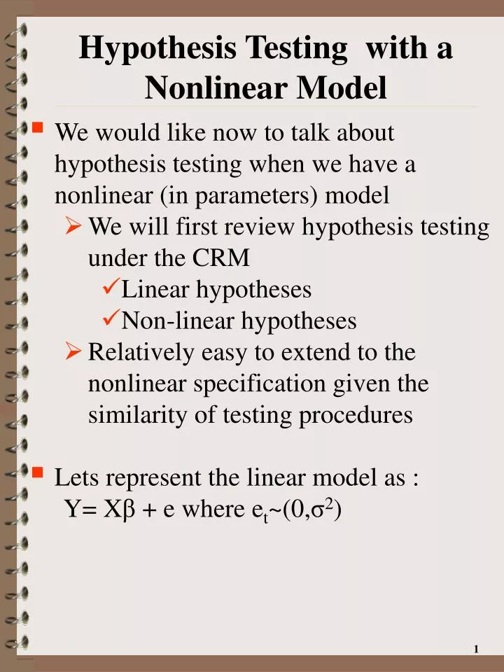
Hypothesis Testing with a Nonlinear Model. We would like now to talk about hypothesis testing when we have a nonlinear (in parameters) model We will first review hypothesis testing under the CRM Linear hypotheses Non-linear hypotheses

E N D
Hypothesis Testing with a Nonlinear Model • We would like now to talk about hypothesis testing when we have a nonlinear (in parameters) model • We will first review hypothesis testing under the CRM • Linear hypotheses • Non-linear hypotheses • Relatively easy to extend to the nonlinear specification given the similarity of testing procedures • Lets represent the linear model as : Y= Xβ + e where et~(0,σ2) 1
Hypothesis Testing Under The General Linear Model • Lets review the general procedures for testing one or more (J) linearcombination of estimated coefficients • Assume we have a-priori information about the value of β • We can represent this information via a set of J-Linear hypotheses (or restrictions): • In matrix notation 2
Hypothesis Testing Under The General Linear Model known coefficients 3
Hypothesis Testing Under The General Linear Model • Assume we have a model with 5 parameters to be estimated, β0 – β4 • Joint hypotheses: β1=8 and β2=β3 • J=2, K=5 β2 −β3=0 4
Hypothesis Testing Under The General Linear Model • How do we obtain parameter estimates if J hypotheses are true? • Constrained (Restricted) Least Squares estimator of β, βR • bR is the value of β that minimizes: S=(Y-Xβ)'(Y-Xβ) s.t. Rβ=r = e'e s.t. Rβ=r e.g. we act as if H0 are true • S*=(Y-Xβ)'(Y-Xβ)+λ'(r-Rβ) • λ is (J x1) Lagrangian multipliers associated with J-joint hypotheses • We want to choose β such that we minimize SSE but also satisfy the J constraints (hypotheses), βR 5
Hypothesis Testing Under The General Linear Model • Min. S*=(Y-Xβ)'(Y-Xβ) + λ'(r-Rβ) • What and how many FOC’s? • K+J Total FOC’s • K FOC’s for the unknown parameters: • J FOC’s associated with the Lagrangian multipliers: 6
Hypothesis Testing Under The General Linear Model S*=(Y-Xβ)'(Y-Xβ)+λ'(r-Rβ) • What are the FOC’s for minimization? CRM βS • Substitute the above into 2nd set of FOC’s ∂S*/∂λ = (r-RβR) = 0J → 7
Hypothesis Testing Under The General Linear Model • The 1st FOC • Substitute the above expression for λ/2 into the 1st FOC: λ/2 8
Hypothesis Testing Under The General Linear Model • βR is the restricted LS estimator of β as well as the restricted ML estimator • Properties of Restricted Least Squares Estimator • →E(bR) b if Rb r • V(bR) ≤ V(bS) →[V(bS) - V(bR)]is positive semi-definite • diag(V(bR)) ≤ diag(V(bS)) True but Unknown Value 9
Hypothesis Testing Under The General Linear Model • From above, if y is multivariate normal and H0is true • βl,R~ N(β,σ2M*(X'X)-1M*') ~ N(β,σ2M*(X'X)-1) • From previous results, if r-Rβ≠0 (e.g., not all H0 true), estimate of β is biased if we continue to assume r-Rβ=0 Idempotent Matrix ≠0 10
Hypothesis Testing Under The General Linear Model • The variance is the same regardless of he correctness of the restrictions and the biasedness of βR • V(βR)= σ2M*(X'X)-1 • → βR has a variance that is smaller when compared to βs which only uses the sample information. • βR uses exogenous information (e.g. R matrix)→ reduced variability 11
Use of Maximum Likelihood Techniques • In order to develop some test statistics, I need to introduce the concept of the sample’s likelihood function • Lets digress and spend some time on the concept of likelihood functions and maximum likelihood estimation • Then return to the topic of hypothesis testing 12
Use of Maximum Likelihood Techniques • Suppose a single random variable yt has a probability density function (PDF) conditioned on a set of parameters, Θ • Represented as: f(yt|Θ) • This function identifies the data generating process that underlies an observed sample of data • Also provides a mathematical description of the data the process will produce 13
Use of Maximum Likelihood Techniques • Suppose we have a random sample of T-observations on y, (y1,y2,…,yT) • Joint PDF of yi’s • Assume they are iid (independently and identicallydistributed) • →Value of yj does not effect the PDF of yi, j ≠ i,f(yi|yj)=g(yi) • Conditional PDF = marginal PDF • Joint distribution of f(yi,yj) = f(yi|yj)h(yj) = g(yi)h(yj) → joint PDF of two iid RV’s is the product of two marginal PDF’s • Extending this → f(y1,y2,y3,…,yT) = f(y1)f(y2)f(y3)…f(yT) where f(yt) is marginal PDF for tth RV 14
Use of Maximum Likelihood Techniques • Joint PDF of yi’s given they are iid (i.e., independently and identicallydistributed) • Value for a single observation can be represented as: f(yt|Q) where • Qis a K-parameter vector • Q W and Ω is allowable parameter set (i.e., σ2 > 0) • Joint PDF: f(Y| Q)=Tt=1 f(yt|Q) 15
Use of Maximum Likelihood Techniques • We can define theLikelihood Function [l(•)] as being identical to the joint PDF but is a function of parameters given data • The LF is written this way to emphasize the interest in the parameters • The LF is not meant to represent a PDF of the parameters • Often times it is simpler to work with the log of the likelihood function, L: 16
Use of Maximum Likelihood Techniques • Since L(•) is a positive monotonic transformation of original likelihood function • Positive monotonic transformation: A method for transforming one set of numbers into another set of numbers so that the rank order of the original set of numbers is preserved. • →Value(s) of Θ that maximize l(•) will also maximize L(•). 17
Use of Maximum Likelihood Techniques • Identification: Parameter vector, Θ, is identified (estimable) if for any other parameter vector, Θ* ≠ Θ, for same data y, l(Θ*|y) ≠ l(Θ |y) • The Principle of Maximum Likelihood • Choose parameter value(s) that maximize the probability of observing the random sample of the data we have • → Parameter values are conditional to the data we have • Is the representation of the distribution of y accurate of the true distribution 18
Hypothesis Testing Under The General Linear Model • Lets now return back to our discussion of hypothesis testing • The Maximum Likelihood (ML) estimate of Θ is the value Θl that max. l(Θ|y) • Θl is in general a function of y, Θl=Θl(y) • Θl is a random variable and referred to as the ML estimator of Θ • Θl chosen such that • The probability of observing the data we actually observe (y, X) is maximized • This is conditional on assumed functional form of the PDF of the y’s (i.e., Likelihood Function) 19
Hypothesis Testing Under The General Linear Model • Lets define the likelihood ratio (LR) as • LR≡lU*/lR* • lU*=Max [l(|y1,…,yT); =(β, σ)] = unrestricted maximum likelihood function • lR*=Max[l(|y1,…,yT); • =(β, σ); Rβ=r] = restricted maximum likelihood function • Because we are restricting the parameter space → LR= lU*/lR*≥ 1 • Fewer values available for β, σ2 • Cannot do any better than lU* Allowable values Could be g(β)=0 20
Hypothesis Testing Under The General Linear Model LR≡lU*/lR* H0: Rβ = r • If lU* is large relative to lR* • → data shows evidence restrictions (hypotheses) are not true (i.e., reject null hypothesis) • Changes the l* value • How much should LR exceed 1 before we reject H0? • Reject H0 when LR ≥ LRC where LRC is a constant chosen on the basis of the relative cost of the Type I vs. Type II errors • Given assumed LR distribution • When implementing the LR Test you need to know dependent variable PDF • Determines the test statistic density 21
Hypothesis Testing Under The General Linear Model y=Xβ + e • From previous results we have: Rβ = r Note: We obtained the above without any assumption about the error term distribution 22
Hypothesis Testing Under The General Linear Model • A continuous random variable yt that has a normal distribution with mean μ and variance σ2 where • -∞ < μ < ∞ • σ2 > 0 • yt has the PDF: • Lets extend this to the CRM, y = Xβ + ε where ε~N(0,σIT) conditional mean 23
Hypothesis Testing Under The General Linear Model • The unrestricted total sample likelihood function (assuming a normal distribution) can be represented via the following: • The restricted likelihood function (incorporating the joint hypotheses) can be represented via the following 24
Hypothesis Testing Under The General Linear Model • Taking the ratio of the two likelihood functions: • Define LR* via the following: • LR* is a monotonic increasing function of LR LR=lU/lR et~N(0,σ2) 25
Hypothesis Testing Under The General Linear Model • What are the distributional characteristics of LR*? • Will address this in a bit • We can derive alternative specifications of LR test statistic • LR*=(SSER-SSEU)/(Js2U) [Ver. 1] • LR*=[(Rbe-r)′[R(X′X)-1R′]-1 (Rbe-r)]/(Js2U)[Ver. 2] • LR*=[(bR-be)′(X′X)(bR-be)]/(Js2U) [Ver. 3] βe =βS=βl 26
Hypothesis Testing Under The General Linear Model • We can derive alternative specifications of LR test statistic • →LR* = (2/T – 1)(T-K)/J • →With σe2 = σl2 = σS2 where • →LR* = [(σR2/σe2) – 1](T-K)/Jwhere • → 27
Hypothesis Testing Under The General Linear Model • With • → • T drops out of σ’s • →(Ver 1) 28
Hypothesis Testing Under The General Linear Model • Remember we have: R = S+ (XX)-1 R[R (XX)-1R]-1 [r – RS] • Define eR = y – XR and eU = y – XS • eR = y–X[βS+(XX)-1R[R(XX)-1 R]-1(r–RβS)] = y–XβS– X(X′X)-1R[R (XX)-1R]-1(r–RβS) • = eU – X(XX)-1R[R(XX)-1R]-1(r–RβS) • where eU = unrestricted error • With SSER = eReR, eR = y – XR • SSER = • {eU – X(XX)-1R[R(XX)-1R]-1(r–RβS)}* • {eU – X(XX)-1R[R(XX)-1R]-1(r–RβS)} • = eUeU + (RS–r)[R (XX)-1R]-1(RS–r) • (After some simplification, JHGLL • p. 258) 29
Hypothesis Testing Under The General Linear Model eReR = eUeU + (RS–r)[R (XX)-1R]-1(RS–r) • SSEU = eU′eU • SSER – SSEU = (RS– r)[R(XX)-1R]-1(RS – r) • Lets now substitute the above into the numerator of (Ver.1) of LR* to create (Ver.2) of LR* (Ver.2) 30
Hypothesis Testing Under The General Linear Model • Again we have: R = S+ (XX)-1R[R (XX)-1R]-1 [r – RS] • Lets multiply both sides by X • X(βR–βS) = X(XX)-1R[R(XX)-1R]-1 [r – RβS] • Pre-multiplying both by their transpose: (βR–βS) XX (βR–βS)= • {(r–RβS)[R(XX)-1R]-1R(XX)-1X} • {X(XX)-1R[R(XX)-1R]-1[r–βS]} • =(r–RβS)[R(XX)-1R]-1(r–RβS) = • SSER – SSEU (from Ver.2 above) • Substitute the above into (Ver.1) (Ver.3) 31
Hypothesis Testing Under The General Linear Model • What are the distributional characteristics of all versions of LR* (JHGLL p. 255)? • We know that • Given the above normality and from page 52 of JHGLL, the following holds Given that it is a quadratic form of a normal RV True Values 32
Hypothesis Testing Under The General Linear Model • Given the definition of σ2U we know the following holds: • Refer to p.226, eq. 6.1.18 and p.52, eq. 2.5.18 in JHGLL • Q1 and Q2 are independently distributed • From page 51 of JHGLL • The ratio of two independent RV’s, e.g. Q1 and Q2 • Each distributed 2 with df1 and df2 degrees of freedom, respectively • The ratio will be distributed Fdf1,df2 where 33
Hypothesis Testing Under The General Linear Model • If the Null Hypotheses are true: • This implies that under the null hypothesis, Rβ=r, LR* ~ FJ,T-K • J = # of Hypotheses • K= # of Parameters • (including intercept) 34
Hypothesis Testing Under The General Linear Model • Proposed Test Procedure • Choose a = P(reject H0| H0 true) = P(Type-I error) • Calculate the test statistic LR* based on sample information • Find the critical value LRcrit in an F-table such that: a = P(F(J, T – K)³ LRcrit), where α = P(reject H0| H0 true) f(LR*) α = P(FJ,T-K ≥ LRcrit) LRcrit α 35
Hypothesis Testing Under The General Linear Model • Proposed Test Procedure • Choose a = P(reject H0| H0 true) = P(Type-I error) • Calculate the test statistic LR* based on sample information • Find the critical value LRcrit in an F-table such that: a = P(F(J, T – K)³ LRcrit), where α = P(reject H0| H0 true) • Reject H0 if LR* ³ LRcrit • Don’t reject H0 if LR* < LRcrit 36
Hypothesis Testing Under The General Linear Model • A side note: How do you estimate the variance of a linear function of estimated parameters from the linear model? • Suppose you have the following model: FDXt = β0 + β1Inct + β2 Inc2t + et • FDX= food expenditure • Inc=household income • Want to estimate the impacts of a change in income on expenditures. • Use an elasticity measure evaluated at mean of the data 37
Hypothesis Testing Under The General Linear Model FDXt = β0 + β1Inct + β2 Inc2t + et data means • Income Elasticity (Γ) is: • How do you calculate the variance of Γ? • In general as noted by JHGLL, p.41: • If a0,a1,…,an are constants and X1,…,Xn are random variables, then • →var(a0 + a1X1)=a12var(X1) and var(X1 ± X2)=var(X1)+var(X2) ± 2cov(X1,X2) Given a linear (parameters) model and an intercept the regression model goes through data means 38
Hypothesis Testing Under The General Linear Model • Thus the variance of a sum (difference) of random variables equals the sum of the variances plus 2 times the covariance • If the Xi’s are statistically independent → cov(Xi,Xj)=0 • → if independent, the variance of a sum of the random variables is the sum of the variances 39
Hypothesis Testing Under The General Linear Model FDXt = β0 + β1Inct + β2 Inc2t + et data means • Income Elasticity (Γ) is: • How do you calculate the variance of Γ? • The above can be represented as Γ=α′W where Wis a vector of RV’s which in this case are parameters and a vector of constants, α • From the results obtained from JHGLL p. 40, we have that σ2(X'X)-1 40
Hypothesis Testing Under The General Linear Model • This implies var(Γ) is: (1 x 3) σ2(X'X)-1 (3 x 3) (3 x 1) Due to 0 Rij value (1 x 1) 41
Hypothesis Testing Under The General Linear Model • Example of Estimation of Single Output Production Function • Example 5.2, Greene, pp: 124-126 • SIC-33: Primary Metals • Cross-Sectional • VA=f(Labor, Capital) • 27 observations 42
Hypothesis Testing Under The General Linear Model 43
Hypothesis Testing Under The General Linear Model • Example of Estimation of Production Function • Cobb-Douglas specification • Translog Functional Form • Cobb-Douglas H0: β3= β4= β5=0 44
Hypothesis Testing Under The General Linear Model • Estimated Coefficients Adj. R2=0.944 45
Hypothesis Testing Under The General Linear Model • Coefficient on lnK < 0 (β2 = -1.8931) • Does this mean that its output elasticity (ψY,K ≡ ∂lnY/∂lnK) is negative? • ψY,K=β2 + β4lnK + β5lnL 46
Hypothesis Testing Under The General Linear Model • Using mean of the natural logarithm of inputs → ψY,K=0.5425 • Note, another point of evaluation could have been at the natural logarithm of the means: • Is ψY,K in fact positive? • Var(ψY,K)=W'ΣβSW • ΣβS is the full 6x6 parameter covariance matrix (1 x 1) β0 β2 β4 β1 β3 β5 47
Hypothesis Testing Under The General Linear Model • Var(ψY,K)=W'ΣβSW=0.01259 • H0: ψY,K = 0, H1: ψY,K > 0 • t.025,22 = 2.074 (critical value) • = Ψstd. dev. • t=0.5425/0.1122= 4.84 • Reject H0 • Conclude that the output elasticity for capital is positive 48
Asymptotic Hypothesis Tests and the Linear Model • Asymptotic Tests (i.e., t → ∞) H0: Rβ = r H1: Rβ≠ r • In general, as T→∞, J x FJ,T-K≈χ2J tT-K≈N(0,1) • → If equation error term not normally distributed and have a “large” number of observations→ joint hypothesis test should be based on J*LR*~c2J (Greene:127-131, JHGLL:268-270) • Define Ver. 2 of LR* Could have used any of the LR* versions 49
Asymptotic Hypothesis Tests and the Linear Model • Proposed Asymptotic Test Procedure: • Choose α = P(Reject H0|H0 true) = P(Type I Error) • Estimate LR** =J x LR* based on the sample information • Find the critical value of such that a=P(c2J >c2J,C) • Reject H0 if LR**>c2J,C, • Do not reject H0 if LR**< c2J,C 50