Download
1 / 68
680 likes | 858 Vues
cs242. Parallelism in Haskell. Kathleen Fisher. Reading: A Tutorial on Parallel and Concurrent Programming in Haskell Skip Section 5 on STM. Thanks to Simon Peyton Jones, Satnam Singh, and Don Stewart for these slides. . The Grand Challenge.

E N D
cs242 Parallelism in Haskell Kathleen Fisher Reading: A Tutorial on Parallel and Concurrent Programming in Haskell Skip Section 5 on STM Thanks to Simon Peyton Jones, Satnam Singh, and Don Stewart for these slides.
The Grand Challenge • Making effective use of multi-core hardware is the challenge for programming languages now. • Hardware is getting increasingly complicated: • Nested memory hierarchies • Hybrid processors: GPU + CPU, Cell, FPGA... • Massive compute power sitting mostly idle. • We need new programming models to program new commodity machines effectively.
Candidate models in Haskell Explicit threads Non-deterministic by design Monadic: forkIO and STM Semi-implicit parallelism Deterministic Pure: par and pseq Data parallelism Deterministic Pure: parallel arrays Shared memory initially; distributed memory eventually; possibly even GPUs… main :: IO () = do { ch <- newChan ; forkIO (ioManagerch) ; forkIO (worker 1 ch) ... etc ... }
Parallelism vs Concurrency • A parallel program exploits real parallel computing resources to run faster while computing the same answer. • Expectation of genuinely simultaneous execution • Deterministic • A concurrent program models independent agents that can communicate and synchronize. • Meaningful on a machine with one processor • Non-deterministic
Haskell Execution Model “Thunk” for fib 10 Pointer to the implementation • 1 • 1 Values for free variables • 8 • 10 Storage slot for the result • 9 • fib 0 = 0 • fib 1 = 1 • fib n = fib (n-1) + fib (n-2) • 5 • 8 • 5 • 8 • 3 • 6
Functional Programming to the Rescue? • No side effects makes parallelism easy, right? • It is always safe to speculate on pure code. • Execute each sub-expression in its own thread? • Alas, the 80s dream does not work. • Far too many parallel tasks, many of which are too small to be worth the overhead of forking them. • Difficult/impossible for compiler to guess which are worth forking. Idea: Give the user control over which expressions might run in parallel.
The parcombinator par :: a -> b -> b x `par` y • Value (ie, thunk) bound to x is sparked for speculative evaluation. • Runtime may instantiate a spark on a thread running in parallel with the parent thread. • Operationally, x `par` y = y • Typically, x is used inside y: • All parallelism built up from the parcombinator. • blurRows `par` (mix blurColsblurRows)
The meaning of par • par does not guarantee a new Haskell thread. • It hints that it would be good to evaluate the first argument in parallel. • The runtime decides whether to convert spark • Depending on current workload. • This allows par to be very cheap. • Programmers can use it almost anywhere. • Safely over-approximate program parallelism.
Example: One processor x `par` (y + x) y y is evaluated x is evaluated x x x is sparked x fizzles
Example: Two Processors x `par` (y + x) P1 P2 y y is evaluated on P1 x x is taken up for evaluation on P2 x x is sparked on P1
Model: One Processor • No extra resources, so spark for f fizzles.
No parallelism? • Main thread demands f, so spark fizzles.
A second combinator: pseq pseq :: a -> b -> b x `pseq` y • pseq: Evaluate x in the current thread, then return y. • Operationally, • With pseq, we can control evaluation order. x `pseq` y = bottom if x -> bottom = y otherwise. e `par` f `pseq` (f + e)
ThreadScope • ThreadScope (in Beta) displays event logs generated by GHC to track spark behavior: Thread 1 Thread 2 (Idle) f `par` (f + e) Thread 1 Thread 2 (Busy) f `par` (e + f)
Sample Program • The fib and sumEuler functions are unchanged. fib :: Int -> Int fib 0 = 0 fib 1 = 1 fib n = fib (n-1) + fib(n-2) sumEuler :: Int -> Int sumEulern = … in ConcTutorial.hs … parSumFibEulerGood :: Int -> Int -> Int parSumFibEulerGood a b = f `par` (e `pseq` (f + e)) where f = fib a e = sumEulerb
Strategies Performance Numbers
Summary: Semi-implicit parallelism • Deterministic: • Same results with parallel and sequential programs. • No races, no errors. • Good for reasoning: Erase the parcombinator and get the original program. • Relies on purity. • Cheap: Sprinkle par as you like, then measure with ThreadScope and refine. • Takes practice to learn where to put par and pseq. • Often good speed-ups with little effort.
Candidate Models in Haskell Explicit threads Non-deterministic by design Monadic: forkIO and STM Semi-implicit Deterministic Pure: par and pseq Data parallelism Deterministic Pure: parallel arrays Shared memory initially; distributed memory eventually; possibly even GPUs… main :: IO () = do { ch <- newChan ; forkIO (ioManagerch) ; forkIO (worker 1 ch) ... etc ... } f :: Int -> Int fx = a `par` b`pseq` a + b where a = f1 (x-1) b = f2 (x-2)
Road map Multicore Parallel programming essential • Task parallelism • Each thread does something different. • Explicit: threads, MVars, STM • Implicit: par & pseq Data parallelism Operate simultaneously on bulk data • Massive parallelism • Easy to program • Single flow of control • Implicit synchronisation Modest parallelism Hard to program
Data parallelism Flat data parallel Apply sequential operation to bulk data Nested data parallel Apply parallel operation to bulk data • The brand leader (Fortran, *C MPI, map/reduce) • Limited applicability (dense matrix, map/reduce) • Well developed • Limited new opportunities • Developed in 90’s • Much wider applicability (sparse matrix, graph algorithms, games etc) • Practically un-developed • Huge opportunity
Flat data parallel Widely used, well understood, well supported BUT: something is sequential. Single point of concurrency Easy to implement: use “chunking” Good cost model foreachi in 1..N { ...do something to A[i]... } P1 P2 P3 1,000,000’s of (small) work items
Nested data parallel Main idea: Allow “something” to be parallel. Now the parallelism structure is recursive, and un-balanced. Still good cost model. Hard to implement! foreachi in 1..N { ...do something to A[i]... } Still 1,000,000’s of (small) work items
Nested DP is great for programmers • Fundamentally more modular. • Opens up a much wider range of applications: • Divide and conquer algorithms (e.g. sort) • Graph algorithms (e.g. shortest path, spanning trees) • Sparse arrays, variable grid adaptive methods (e.g. Barnes-Hut) • Physics engines for games, computational graphics (e.g. Delauny triangulation) • Machine learning, optimization, constraint solving
Nested DP is tough for compilers ...because the concurrency tree is both irregular and fine-grained. But it can be done! NESL (Blelloch 1995) is an existence proof. Key idea: “Flattening” transformation: Nested data parallel program (the one we want to write) Flatdata parallel program (the one we want to run) Compiler
Data Parallel Haskell • NESL (Blelloch)A mega-breakthrough but: • specialized, prototype • first order • few data types • no fusion • interpreted • Substantial improvement in • Expressiveness • Performance • Shared memory initially • Distributed memory eventually • GPUs anyone? Haskell • broad-spectrum, widely used • higher order • very rich data types • aggressive fusion • compiled Not a special purpose data-parallel compiler! Most support is either useful for other things, or is in the form of library code.
Array comprehensions [:Float:] is the type of parallel arrays ofFloat vecMul :: [:Float:] -> [:Float:] -> Float vecMul v1 v2 = sumP [: f1*f2 | f1 <- v1 | f2 <- v2 :] An array comprehension: “the array of all f1*f2 where f1 is drawn from v1 and f2 from v2 in lockstep.” sumP :: [:Float:] -> Float Operations over parallel array are computed in parallel; that is the only way the programmer says “do parallel stuff.” NB: no locks!
Sparse vector multiplication A sparse vector is represented as a vector of (index, value) pairs: [:(0,3),(2,10):]instead of [:3,0,10,0:]. sDotP:: [:(Int,Float):] -> [:Float:] -> Float sDotPsvv = sumP [: f * (v!i) | (i,f) <- sv :] v!i gets the ithelement of v sDotP [:(0,3),(2,10):][:2,1,1,4:] = sumP [: 3 * 2, 10 * 1 :] = 16 Parallelism is proportional to length of sparse vector.
Sparse matrix multiplication A sparse matrix is a vector of sparse vectors: [:[:(1,3),(4,10):], [:(0,2),(1,12),(4,6):]:] smMul :: [:[:(Int,Float):]:] -> [:Float:] -> Float smMulsmv = sumP [:sDotPsvv | sv <- sm :] Nested data parallelism here!We are calling a parallel operation, sDotP, on every element of a parallel array, sm.
Example: Data-parallel Quicksort sort :: [:Float:] -> [:Float:] sort a = if (lengthPa <= 1) then a else sa!0 +:+ eq +:+ sa!1 where p= a!0 lt = [: f | f<-a, f<p:] eq = [: f | f<-a, f==p:] gr = [: f | f<-a, f>p:] sa = [: sort a | a <- [:lt,gr:] :] Parallel filters 2-way nested data parallelism here.
How it works Step 1 sort sort sort Step 2 Step 3 sort sort sort ...etc... • All sub-sorts at the same level are done in parallel. • Segment vectors track which chunk belongs to which sub problem. • Instant insanity when done by hand.
Example: Parallel Search type Doc = [: String :] -- Sequence of words type Corpus = [: Doc :] search :: Corpus -> String -> [: (Doc,[:Int:]):] Find all Docs that mention the string, along with the places where it is mentioned (e.g. word 45 and 99)
Example: Parallel Search type Doc = [: String :] type Corpus = [: Doc :] search :: Corpus -> String -> [: (Doc,[:Int:]):] wordOccs :: Doc -> String -> [: Int :] Find all the places where a string is mentioned in a document (e.g. word 45 and 99) .
Example: Parallel Search type Doc = [: String :] type Corpus = [: Doc :] search :: Corpus -> String -> [: (Doc,[:Int:]):] search dss = [: (d,is) | d <- ds , let is = wordOccsds , not (nullP is) :] wordOccs :: Doc -> String -> [: Int :] nullP :: [:a:] -> Bool
Example: Parallel Search type Doc = [: String :] type Corpus = [: Doc :] search :: Corpus -> String -> [: (Doc,[:Int:]):] wordOccs :: Doc -> String -> [: Int :] wordOccs d s = [: i | (i,si) <- zipP positions d , s == si :] where positions :: [: Int :] positions = [: 1..lengthP d :] zipP :: [:a:] -> [:b:] -> [:(a,b):] lengthP :: [:a:] -> Int
Hard to implement well! • Evenly chunking at top level might be ill-balanced. • Top level alone might not be very parallel. Corpus Documents
The flattening transformation • Concatenate sub-arrays into one big, flat array. • Operate in parallel on the big array. • Segment vector tracks extent of sub-arrays. etc… • Lots of tricksy book-keeping! • Possible to do by hand (and done in practice), but very hard to get right. • Blelloch showed it could be done systematically.
Fusion Flattening enables load balancing, but it is not enough to ensure good performance. Consider: Bad idea: Generate [: f1*f2 | f1 <- v1 | f2 <-v2 :] Add the elements of this big intermediate vector. Good idea: Multiply and add in the same loop. That is, fusethe multiply loop with the add loop. Very general, aggressive fusion is required. vecMul :: [:Float:] -> [:Float:] -> Float vecMul v1 v2 = sumP [: f1*f2 | f1 <- v1 | f2 <- v2 :]
Implementation Techniques Four key pieces of technology: • Vectorization • Specific to parallel arrays • Non-parametric data representations • A generically useful new feature in GHC • Distribution • Divide up the work evenly between processors • Aggressive fusion • Uses “rewrite rules,” an old feature of GHC } Flattening Main advance: an optimizing data-parallel compiler implemented by modest enhancements to a full-scale functional language implementation.
Step 0: Desugaring • Rewrite Haskell source into simpler core, e.g, removing array comprehensions: sDotP :: [:(Int,Float):] -> [:Float:] -> Float sDotPsvv = sumP [: f * (v!i) | (i,f) <- sv :] sDotPsvv = sumP (mapP (\(i,f) -> f * (v!i)) sv) sumP :: Num a => [:a:] -> a mapP :: (a -> b) -> [:a:] -> [:b:]
Step 1: Vectorization • Replace scalar function f by the lifted (vectorized) version, written f^. svMul :: [:(Int,Float):] -> [:Float:] -> Float svMulsvv = sumP (mapP (\(i,f) -> f * (v!i)) sv) svMulsvv = sumP (snd^ sv *^ bpermutePv (fst^ sv)) sumP :: Num a => [:a:] -> a *^ :: Num a => [:a:] -> [:a:] -> [:a:] fst^ :: [:(a,b):] -> [:a:] snd^ :: [:(a,b):] -> [:b:] bpermuteP :: [:a:] -> [:Int:] -> [:a:]
Vectorization: Basic idea mapPfv f^ v f :: T1 -> T2 f^ :: [:T1:] -> [:T2:] -- f^ = mapPf • For every function f, generate its lifted version, named f^. • Result: A functional program, operating over flat arrays, with a fixed set of primitive operations *^, sumP, fst^, etc. • Lots of intermediate arrays!
Vectorization: Basic idea f :: Int -> Int fx = x + 1 f^ :: [:Int:] -> [:Int:] f^ xs= xs+^ (replicateP (lengthPxs) 1) replicateP :: Int -> a -> [:a:] lengthP :: [:a:] -> Int
Vectorization: Problem • How do we lift functions that have already been lifted? f :: [:Int:] -> [:Int:] fxs= mapPgxs= g^xs f^ :: [:[:Int:]:] -> [:[:Int:]:] f^xss= g^^xss--??? Yet another version of g???
Vectorization: Key insight First concatenate, then map, then re-split f :: [:Int:] -> [:Int:] fxs= mapPgxs= g^xs f^ :: [:[:Int:]:] -> [:[:Int:]:] f^xss= segmentPxss(g^ (concatPxss)) concatP :: [:[:a:]:] -> [:a:] segmentP :: [:[:a:]:] -> [:b:] -> [:[:b:]:] Shape Flat data Nested data Payoff: f and f^ are enough. No f^^.
Step 2: Representing arrays [:Double:]Arrays of pointers to boxed numbers are Much Too Slow. [:(a,b):] Arrays of pointers to pairs are also Much Too Slow. Idea! Select representation of array based on its element type… ...
Step 2: Representing arrays • Extend Haskell with construct to specify families of data structures each with a different implementation. AP data family [:a:] data instance [:Double:] = ADIntByteArray data instance [:(a, b):] = AP [:a:] [:b:] [POPL05], [ICFP05], [TLDI07]