Download
1 / 71
730 likes | 1.25k Vues
Sub electron noise readout for scientific CCDs. Research Techniques Seminar September 14, 2010. Gustavo Cancelo. CCD low noise readout: Juan Estrada. Ken Treptow . Gullermo Fernandez Moroni . Gustavo Cancelo. Tom Diehl. Kevin Kuk . Ted Zmuda . DES collaboration:. Outline:.

E N D
Sub electron noise readout for scientific CCDs Research Techniques Seminar September 14, 2010 Gustavo Cancelo
CCD low noise readout: • Juan Estrada. • Ken Treptow. • Gullermo Fernandez Moroni. • Gustavo Cancelo. • Tom Diehl. • Kevin Kuk. • Ted Zmuda. • DES collaboration:
Outline: • Brief introduction to CCDs. • Applications. • Low noise readout. • Future work. • CCD full well issue. • Outreach.
Charge Coupled Devices (CCD) Most scientific CCDs: Low resistivity, thinned down to 20µ to increase depletion. n-channel: better charge mobility but higher dark current. LBNL CCDs used for DES DECam: High resistivity, 250µ thick High QE in near infrared. Z>1 1g of mass, good for direct DM search. p-channel, better than n-channel for space telescopes
Charge Coupled Devices (CCD) Photon Transfer Curve (PTC) • Photon Transfer Curve: • Full well • Readout gain • Pixel and dark current non uniformity • more... Potential well The location and size of the well’s maximum potential is a function of the pixel layout, Si process, doping concentrations and externally applied voltages.
Outline: • Brief CCD introduction. • Applications. • Low noise readout. • Future work. • Full well issue. • Outreach.
Dark Energy Camera (DECam) New wide field imager for the Blanco telescope (largest focal plane in the southern hemisphere) Largest CCD project at FNAL. DECam is being built at FNAL including CCD packaging, full characterization, readout electronics. CCD facilities at SiDet and 5+ years of experience positions FNAL as a leader for this task. Blanco 4m Telescope Cerro Tololo, Chile Mechanical Interface of DECam Project to the Blanco CCD Readout Filters Shutter Hexapod Optical Lenses Focal plane with 74 CCDs (~600 Mpix). All the scientific detectors in hand, packaged and characterized at FNAL.
DECam has allowed us to build at FNAL a powerful CCD lab closely monitoring production of dies for more than 2 years, giving quick feedback on performance developed CCD package for focal plane that meets scientific requirements produced/tested 240+ CCDs like an efficient factory designed and build readout electronics for a large focal plane the experience building silicon trackers transferred nicely to this project. The work in this talk has been possible thanks to this CCD lab.
Overlap with South Pole Telescope Survey (4000 sq deg) Survey Area Connector region (800 sq deg) Overlap with SDSS Stripe 82 for calibration (200 sq deg) Dark Energy Survey optimized to measure the equation of state parameter w for Dark Energy. Relation between pressure and density. Galaxy Cluster counting (collaboration with SPT, see next slides) 20,000 clusters to z=1 with M>2x10¹⁴Msun Spatial clustering of galaxies (BAO) 300 million galaxies to z ~ 1 Weak lensing 300 million galaxies with shape measurements over 5000 sq deg Supernovae type Ia (secondary survey) ~1100 SNeIa, to z = 1 error ellipse DES expects factor of 5 improvement over current experiments
DES upgrade DECam estimates redshift from the colors of the objects. FNAL scientists are now planning a spectrograph to complement DES data. The CCD work in astrophysics at FNAL is NOT over. multi object spectrograph using many DECam parts X000 fibers 4 DES filters colors change as galaxy moves in z several spectrographs
Beyond DES --- LSST next big survey, to be built in the mountain next to DECam. Huge CCD camera (3.2 Gpix) with a more demanding electronic performance (faster readout and lower noise!) slide by P. O’Connor (BNL) It makes a lot of sense for FNAL to get involved in this. In this talk I will show you that we are now meeting the LSST readout requirements. In a few weeks we will be testing a detector with almost the correct format for LSST. The CCD work in astrophysics at FNAL is NOT over.
Limited by detection threshold. Most experiments can not lower threshold because of the electronic readout noise in their detectors. Room for CCDs! from Petriello & Zurek 0806.3989 limited by exposure mass (need bigger detector) Another CCD application: DAMIC SUSY models Ideal, threshold set below 1e- (i.e. noise below 0.2e-)
7.2 eV noise ➪ low threshold (~0.036 keVee) • 250 μm thick ➪ reasonable mass (a few grams detector) DECAM CCDs are good for low threshold DM search Two features: CCDs are readout serially (2 outputs for 8 million pixels). When readout slow, these detectors have a noise below 2e- (RMS). This means anRMS noise of 7.2 eV in ionization energy! The devices are “massive”,1 gram per CCD. Which means you could easily build ~10 g detector. DECam would is a 70 g detector. σ = 2e
One good reason to look for low mass dark matter : The DAMA/LIBRA result Bernabei et al, 2008 ~8 σ detection of annual modulation consistent with the phase and period expected for a low mass dark matter particle (~7 GeV) consistent with recent COGENT results.
Particle detection with CCDs muons, electrons and diffusion limited hits. nuclear recoils will produce diffusion limited hits
thanks to our low noise we have the best result in the world and we are reaching the DAMA region COGENT 1 gram of Si DAMIC CRESST DAMA w chan. CCD copper dewar inside lead shield. DAMA w/o chan The low noise readout system would allow to set a lower threshold for this search. Number of recoils increase al low energies.
Neutrino coherent scattering: • CCD threshold <100 eV (goal ~10 to 15eV) • SM cross section is relatively large, the challenges are detector sensitivity and background control. • SM and new physics. • Help understand how to study supernovae neutrinos. • Monitoring of nuclear reactors. ☚ we are here ~100 cpd/keV/kg @ 100eV noise reduction event rate ( cpd/keV/kg) lower noise in this case means that we can see the recoils with over a larger background Expected rate for nuclear recoils ~30m from the center of a 3GW reactor. (From the Texono collaboration) recoil energy (keV)
Neutron Imager : more CCD R&D at FNAL • Neutron imaging is complementary of x-ray imaging, sometimes the only option • Cargo scanning. • Nuclear technology. • Archeology, paleontology. • Materials research. ~1mm resolution this is done all the time with CCD, but we want to skip the scintillator to improve resolution.
Neutron Imager : more CCD R&D at FNALmotivated by exchange with neutron physicists during ICFA school borated CCD readout this is done all the time with CCD, but we want to skip the scintillator to improve resolution. our spatial resolution will be the position of the position resolution of measuring alphas in the CCDs pixels.
alphas in CCDs using 241Am thanks to the plasma effect the alphas are clearly identifiable in our the CCDs, and we can measure their full energy. The lower energy photons coming from the source can be easily separated. This is interesting for other reasons, there is not much experience with alphas in CCDs and they allow for a good measurement of the space charge effects in silicon. so we are now setting a first test with a borated plate over the CCD. If things look good we will try to deposit Boron on the surface of the detector (or maybe the detector package). Working closely with neutron physicist on this project.
Outline: • Brief CCD introduction. • Applications. • Low noise readout. • Future work. • Full well issue. • Outreach.
CCD architecture CCD array CCD transfer function • CCDs have one or more arrays of small pixels. • DES CCD have 8Mpixels of 15 x 15 microns. • Pixels are readout serially through one or more video amplifiers. • Pixel charge shifts vertically into an horizontal register and then the horizontal register is readout serially. • Most CCD noise comes from the video and external readout. • When cold at ~-100˚C, the dark current is negligible. • Charge transfer efficiency is better than 99.99% (i.e. 1 ppm charge diffusion). Output video circuit CCD readout noise CCD gain defined in digital units per e- (ADU/e-)
CCD Images FITS image: Each pixel is a n-bit digital representation of the pixel charge. Fragment of video output Pedestal Pixel T T Correlated Double Sampling (CDS) CDS can be done in the analog (continuous) or digital (sampled) domain. for an integration window T Where sigi(t) is the i-th image pixel and pedi(t) is the pedestal.
CCD video output Reset pulses are ~ 50,000 e- 1/f + WGN Reset feed through noise Reset pulses (different height) Low frequency correlation One pedestal and one pixel value Summing well clock feed trough buried in noise.
CCD noise • CCD noise measured by the LBNL designers using a test board. • 1/f noise up to 50 KHz. • WGN at higher frequencies. • VREF and VDD power supply noise is critical. • Pulsed signals: RESET and summing well noise change the baselines.
CCD noise and CCD readout noise • CCD noise • Dark current is negligible at cryogenic temperatures. • Mainly shot noise from signal (Poisson). • CCD readout noise: • 1/f noise. • Thermal (shot) noise (WGN), limited by high bandwidth amplifiers and external LPF. • CCD readout system noise sources • Power supplies. • Readout amplifier chain. • Analog to digital converter. • EMI.
Video fragment: Npix pixels and Npix pedestals long. Pixeli Pedestal i Pedestal i+1 Pixel i+1 Correlated Double Sampling (CDS) Integration intervals: t4-t3 = t2-t1 = T x(n) = s(n) + n(n) + w(n) s(n) pedestals and pixels n(n) correlated noise w(n) white Gaussian noise For the white and Gaussian noise w ~ N(0,σ²), the CDS is the optimum estimator. but It actually grows for longer T because the 1/f noise grows exponentially as f->0.
CCD noise measured with the Monsoon system • 3.5e- at 10μs. • Below 2e- for T > 40μs. • The noise increases for long pixel observations T > 70 us. • Meets comfortably DeCam specs of 10e- at 4μs σ = 3.5e This is good, but how can we do better?
CCD video noise spectrum • System noise 5 to 10 times higher than CCD noise. • Resonances indicate EMI induced noise. • Too much low frequency content. • CCD device noise: • WGN of 10µV over (10Hz-100KHz), equivalent to 4e-/sample RMS. CCD system noise: 20 to 30 e-/sample RMS.
CCD video noise spectrum • More resonances at 60 and 120 Hz induced by AC power. 120Hz resonances • EMI: • Conductive noise. • E and M coupled noise. • We can’t change the interference source, but we can move the sensitive system.
Correlated double sampling (CDS) Alternative method • Sample the video output. • N samples of the pedestal and the pixel value every T. • Digital Signal Process the data using digital filters and estimators. • Advantage: • Lower noise. • Disadvantage: • More computing resources. • Advantages: • Generates a single data point per pixel. • Pedestal subtraction. • The CDS filtering is implemented by a simple analog circuit. • Disadvantage: • One sample/pixel eliminates the possibility of signal processing.
24 bit Σ-Δ ADC based readout system CDS of 50Ω terminated input FFT of 50Ω terminated input 1e- at 1µs 0.3e- at 10µs Gain: 35 ADUs/e- Single sample rms: 1.5e- Output sample rate: 2.5samples/µs. ADC noise spectrum is flat (WGN)
CDS transfer function Tpix Video without noise Correlated noise The CDS filters very low frequency noise close to DC. Minimum noise rejection at f~0.4/TPix. Nulls at f=k/TPix, where k=1,2,3,… Better filtering for higher frequencies. Transfer function maximums follow a |sin(x)/x| decay. f .TPix ? Noise power spectrum Snoise is the WGN (band limited by analog filters) 1/f noise in BW 0 – 10 KHz . Tpixis a “free” parameter
Cumulative CDS transfer function Let’s assume that most of the noise is band limited WGN Noise power If the input power noise is flat and band limited. 90% of the CDS noise is due to low frequency noise (0< fnoise < 1/TPix). If we add 1/f noise 90% of the noise is within 0< fnoise < α/TPix, α<1. Eliminating low frequency noise beyond what CDS can do is interesting: We use estimation. WGN + 1/f WGN only
Cumulative CDS transfer function WGN + 1/f Can we estimate low frequency content and subtract it from the CDS noise? How many low frequency modes do we need to estimate? WGN only Example: Tpix = 10 to 12µs. Data sample: 20 pixels + 20 pedestals long data sets. Estimation of 20 to 30 modes. The first 3 or 4 modes may not be needed. For longer integration times we need mode modes.
2*Npix steps with N total samples, Ns samples per step Pixel i Pedestal i Pedestal i+1 Pixel i+1 Estimator • χ2 estimator, because it does not assume a particular noise model: • Inversion of a large matrix. • Only one time and can be done off-line. • Numeric problems if matrix is too large and rectangular. • Linear model is not orthogonal. Estimation errors are correlated. • Study covariance matrix • Goal: • Implement the estimator and the digital CDS in an FPGA. • FPGAs have a couple hundred multipliers working in parallel at > 100 MHz. s(n) pedestals and pixels n(n) correlated noise w(n) white Gaussian noise signal model: WhereUi(n) is a step (Heaviside) function centered at pixel or pedestal i.
Estimation of correlated noise The idea is that if we know the amplitude and phases of p terms of the correlated noise we can subtract them. Of course we also need to know the pedestal and pixel values si for all i=1…2Npix. Number of parameters to be estimated: p+2Npix. Linear estimation model: where θ is a (p+2Npix)x1 vector H non orthogonal because the step functions are non orthogonal to the Fourier basis. If w~N(0,σ2) is WGN For H orthogonal this is equal to In our case H is not orthogonal, so some estimation errors are larger than others.
We can eliminate the pedestal and pixel values si from the estimation problem. where <x(n)> is the average signal+noise value in each pixel (step function) New linear model: where θ is a px1 vector y(n) x(n) Less parameters need to be estimated. H is better behaved. The CDS of low frequency noise is subtracted from the total CDS of signal+noise.
Digital CDS using the 24 bit ADC 24 bit ADC: Digital CDS Monsoon: analog CDS σ = 3.5e σ = 1.1e The digital CDS using the 24 bit ADC x3 lower in noise at 12µs.
Estimation results Noise in electrons Noise in electrons 0.87e- 0.77e- 30% improvement 35% improvement Can we still do better? What are the limitations of the estimator?
Estimator limitations • We have observed noise minimums at 10 to 12 µs. • Estimation example: • 20 pixels (and 20 pedestals). • 2.5Msamples/s. • 10µs/pix. • Total samples: 1000. • CDS has low gain for the first 5 modes. We may not need them. • We can locate 1/f noise corner frequency at low CDS gain. • The 1/f noise corner ~10KHz. • In our example the first mode is at 2.5KHz. • 1/f occupies 4 to 5 modes. The estimation error is improved if we lower the WGN noise power and/or if we add more samples N.
Lowering the WGN • Most of the WGN comes from power supplies that power the CCD output video (i.e. CCD internal or external amplifiers) and the ADC (i.e. quantization noise). • We showed ADC = 1e- at 1µs, 0.3e- at 10µs, goes with 1/sqrt(N) • Currently, power supply noise is too high and can be improved. • Grounding and shielding noise. Can also be improved. • Lowering the WGN is the first priority because it also improves the parameter estimation. • WGN reduction of 50% is possible. • This is a 0.3e- noise reduction at 10µs.
Estimation errors • Longer observation times may not be the solution: • Increasing the number of samples improves our estimation by 1/sqrt(N). • The 1/f noise moves closer to the maximum of the CDS transfer function. 1/f grows exponentially. • We need to estimate mode low frequency modes. • We need to handle a larger H matrix. Larger numerical errors. • Increasing the sampling rate would be the way to go but we are already using a state of the art ADC.
Covariance of H For an orthogonal matrix the estimation errors are uncorrelated and inversely proportional to the sqrt of the number of samples N. • Estimation errors are much larger for the first few modes (not shown in the plot) . • For the modes 5 to 15 the errors are between 4.5 and 2 times larger. • Lower frequency signals have larger estimation errors. Our H is not orthogonal, how bad conditioned is this matrix compared to an orthogonal matrix? So, we look at CDS weights the errors. Large errors in the first few modes go down significantly.
Estimation results Lowest mode not estimated Noise in electrons 35% improvement
Estimating more modes • Increasing the pixel readout time (e.g. 30µs) • The covariance function coefficients (HTH)-1 of the estimation errors do not increase but we have more parameters to estimate. • The problem is the 1/f noise.
Parameter estimation time consistency Noisy video • The green, blue and red symbols are the estimation parameters for 3 time consecutive data sets. Each data set is 20 pixels long (i.e. 20 pedestals and 20 pixels). • We estimate Fourier coefficients, so we can calculate the amplitude and phase. • The estimated amplitudes of low freq. modes are consistent for modes 5 and above. • The estimation of lower modes (i.e. 1 to 5) are not because they have a large error. • The estimated phases , of course, are different and need to be accounted for. • It means that the statistics on our estimation can be improved by the previous estimations, at least for some time. There are several estimators that do that, such as sequential χ2, ARMA, Wiener, Kalman, etc. 20 pedestals + pixels Green, red and blue are time consecutive data sets.
Do we understand what we see? • At ~12µs we see minimum noise of 1 e- before the estimator and 0.77 e- after applying the estimator. • The ADC noise for 12µs is 0.3 e-. • The rms power supply noise is 700 ADUs (i.e. 20 e-). This gives us 0.7 e- at 12µs. • If we use the flat spectrum noise approximation. The estimation errors are almost uncorrelated and can be added in quadrature using: coeffp= red circles where For 12µs we obtain a σtot = 0.7 e- The expected total error is 0.62 e-. We measure 0.77 e-. The difference is that for the calculations we are using the flat spectrum approximation (i.e. no 1/f, no EMI noise).