Download
1 / 54
540 likes | 694 Vues
Use of Genetic Algorithm for Quantum Information Processing by NMR V.S. Manu and Anil Kumar Centre for quantum Information and Quantum Computing Department of Physics and NMR Research Centre Indian Institute of Science, Bangalore-560012. The Genetic Algorithm. John Holland.

E N D
Use of Genetic Algorithm for Quantum Information Processing by NMR V.S. Manu and Anil Kumar Centre for quantum Information and Quantum Computing Department of Physics and NMR Research Centre Indian Institute of Science, Bangalore-560012
The Genetic Algorithm John Holland Charles Darwin 1866 1809-1882
“Genetic Algorithms are good at taking large, potentially huge, search spaces and navigating them, looking for optimal combinations of things, solutions you might not otherwise find in a lifetime” Here we apply Genetic Algorithm to Quantum Computing and Quantum Information Processing
Quantum Algorithms 1. PRIME FACTORIZATION Classically : exp [2(ln c)1/3(ln ln c)2/3] 400 digit 1010years(Age of the Universe) Shor’s algorithm : (1994) (ln c)3 3 years 2. SEARCHING ‘UNSORTED’ DATA-BASE Classically : N/2 operations Grover’s Search Algorithm : (1997) Noperations 3. DISTINGUISH CONSTANT AND BALANCED FUNCTIONS: Classically : ( 2N-1 + 1) steps Deutsch-Jozsa(DJ) Algorithm : (1992) . 1 step 4. Quantum Algorithm for Linear System of Equation: Harrow, Hassidim and Seth Lloyd; Phys. Rev. Letters, 103, 150502 (2009). Exponential speed-up
Recent Developments 5. Simulating a Molecule: Using Aspuru-Guzik Algorithm (i) J.Du, et. al, Phys. Rev. letters 104, 030502 (2010). Used a 2-qubit NMR System ( 13CHCl3 ) to calculated the ground state energy of Hydrogen Molecule up to 45 bit accuracy. (ii) Lanyon et. al, Nature Chemistry 2, 106 (2010). Used Photonic system to calculate the energies of the ground and a few excited states up to 20 bit precision.
Experimental Techniques for Quantum Computation: 3. Cavity Quantum Electrodynamics (QED) 2. Polarized Photons Lasers 1. Trapped Ions 4. Quantum Dots 5. Cold Atoms 6. NMR 7. Josephson junction qubits 8. Fullerence based ESR quantum computer
Photograph of a chip constructed by D-Wave Systems Inc., designed to operate as a 128-qubitsuperconductingadiabatic quantum optimization processor, mounted in a sample holder. 2011
0 Nuclear Magnetic Resonance (NMR) 1.Nuclear spins have small magnetic moments (I) and behave as tiny quantum magnets. B1 2.When placed in a large magnetic field B0 , they oriented either along the field (|0 state) or opposite to the field (|1 state) . 3.A transverse radiofrequency field (B1) tuned at the Larmor frequency of spins can cause transition from |0 to |1 (NOT Gate by a 1800 pulse). Or put them in coherent superposition (Hadamard Gate by a 900 pulse).Single qubit gates. 4.Spins are coupled to other spins by indirect spin-spin (J) coupling, and controlled (C-NOT) operations can be performed using J-coupling. Multi-qubit gates SPINS ARE QUBITS
Field/ Frequency stability = 1:10 9 DSX 300 AV 700 NMR Research Centre, IISc 1 PPB DRX 500 AV 500 AMX 400
Why NMR? > A major requirement of a quantum computer is that the coherence should last long. > Nuclear spins in liquids retain coherence ~ 100’s millisec and their longitudinal state for several seconds. > A system of N coupled spins (each spin 1/2) form an N qubit Quantum Computer. > Unitary Transform can be applied using R.F. Pulses and J-evolution and various logical operations and quantum algorithms can be implemented.
Achievements of NMR - QIP 10. Quantum State Tomography 11. Geometric Phase in QC 12. Adiabatic Algorithms 13. Bell-State discrimination 14. Error correction 15. Teleportation 16. Quantum Simulation 17. Quantum Cloning 18. Shor’s Algorithm 19. No-Hiding Theorem 1. Preparation of Pseudo-Pure States 2. Quantum Logic Gates 3. Deutsch-Jozsa Algorithm 4. Grover’s Algorithm 5. Hogg’s algorithm 6. Berstein-Vazirani parity algorithm 7. Quantum Games 8. Creation of EPR and GHZ states 9. Entanglement transfer Also performed in our Lab. Maximum number of qubits achieved in our lab: 8 In other labs.: 12 qubits; Negrevergne, Mahesh, Cory, Laflamme et al., Phys. Rev. Letters, 96, 170501 (2006).
NMR sample has ~ 1018 spins. Do we have 1018 qubits? No - because, all the spins can’t be individually addressed. Progress so far Spins having different Larmor frequencies can be individually addressed as many “qubits” One needs resolved couplings between the spins in order to encode information as qubits.
NMR Hamiltonian H = HZeeman + HJ-coupling = wi Izi + Jij Ii Ij Two Spin System (AM) bb = 11 i i < j Weak coupling Approximation wi - wj>> Jij A2= 1M M2= 1A ab = 01 ba = 10 H= wi Izi+ Jij Izi Izj M1= 0A A1= 0M i i < j aa = 00 Spin States are eigenstates A1 M1 A2 M2 Under this approximation all spins having same Larmor Frequency can be treated as one Qubit wM wA
13CHFBr2 An example of a three qubit system. A molecule having three different nuclear spins having different Larmor frequencies all coupled to each other forming a 3-qubit system Homo-nuclear spins having different Chemical shifts (Larmor frequencies) also form multi-qubit systems
3 Qubits 111 011 110 101 010 001 100 000 2 Qubits 1 Qubit CHCl3 11 1 10 01 0 00
Unitary Transforms in NMR • Rational Pulse design. • (using RF Pulses and coupling (J)-evolution) 2. Optimization Techniques U1 Goodness criterion σinitial σfinal σ1 Iterate to minimize C1 C1 = l σ1 –σf l • Various optimization Techniques used in NMR • Strongly Modulated Pulses (SMP) (Cory, Mahesh et. al) • Control Theory (Navin Kheneja et. al (Harvard)) • Algorithmic Technique (Ashok Ajoy et. al) • Genetic Algorithm (Manu)
1. Rational Pulse design. using RF Pulses and coupling (J)-evolution
The two methods Coupling (J) Evolution Transition-selective Pulses Examples 11 I1z+I2z XOR/C-NOT p y I1 I1z+I2x 01 10 x y (1/2J) I1z+2I1zI2y 00 I2 x 1/4J 1/4J I1z+2I1zI2z 11 p I1 01 10 NOT1 I2 p 00
y x -y 11 I1 y x -y I2 y y -x -x I1 I2 I3 01 10 SWAP p1 p3 p2 00 111 p 011 110 101 Toffoli 010 001 100 000 y y -x x non-selective p pulse + a p on 000 001 111 I1 011 110 101 I2 OR/NOR 010 001 100 p I3 000
CNOT GATE 1 2 z y x
Logic Gates Using 1D NMR NOT(I1) C-NOT-2 XOR2 C-NOT-1 XOR1 Kavita Dorai, PhD Thesis, IISc, 2000.
|00> |01> |10> |11> SWAP GATE 1 2 5 3 4 1 2 11 1 01 10 2 00 3 J 4 5
e1 , e2 e2 , e1 1 0 2 11 1 1 01 10 2 00 0 0 0 0 INPUT OUTPUT 1 0 0 1 1 0 0 1 1 1 1 1 p Logical SWAP XOR+SWAP p p1 p2 p3 Kavita, Arvind, and Anil Kumar Phys. Rev. A 61, 042306 (2000).
1 1 2 2 3 3 Toffoli Gate = C2-NOT e1 , e2 , e3 e1 , e2 , e3 (e1e2) ^ Input Output 000 000 001 001 010 010 011 111 100 100 101 101 110 110 111 011 AND Eqlbm. p NAND Toffoli Kavita Dorai, PhD Thesis, IISc, 2000.
Strongly Modulated Pulses (SMP) (Cory, Mahesh et. al)
Adiabatic Satisfibility problem • using Strongly Modulated Pulses Avik Mitra
spins are close (~ kHz) in frequency space In a Homonuclear spin systems Decoherence effects cannot be ignored Pulses are of longer duration Strongly Modulated Pulses circumvents the above problems
F F c b C C I F a • NMR Implementation, using a 3-qubit system. • The Sample. Iodotrifluoroethylene(C2F3I) • Equilibrium Specrum.
Implementation of Adiabatic Evolution mth step of the interpolating Hamiltonian . mth step of evolution operator • Pulse sequence for adiabatic evolution • Total number of iteration is 31 • time needed = 62 ms • (400s x 5 pulses x 31 repetitions)
slope: rf • Strongly Modulated Pulses. Nedler-Mead Simplex Algorithm (fminsearch)
Using ConcatenatedSMPs Duration: Max 5.8 ms, Min. 4.7 ms Avik Mitra et al, JCP, 128, 124110 (2008)
Results for all Boolean Formulae Avik Mitra et al, JCP, 128, 124110 (2008)
Algorithmic Technique (Ashok Ajoy et. al PRL under review) Applied for proving Quantum No-Hiding Theorem by NMR Jharana Rani Samal, Arun K. Pati and Anil Kumar, Phys. Rev. Letters, 106, 080401 (25 Feb., 2011)
Quantum Circuit for Test of No-Hiding Theorem using State Randomization (operator U). H represents Hadamard Gate and dot and circle represent CNOT gates. After randomization the state |ψ> is transferred to the second Ancilla qubit proving the No-Hiding Theorem. (S.L. Braunstein, A.K. Pati,PRL 98, 080502 (2007).
The Randomization Operator is obtained as U = Blanks = 0
Conversion of the U-matrix into an NMR Pulse sequence has been achieved here by a Novel Algorithmic Technique, developed in our laboratory by Ajoy et. al (to be published). This method uses Graphs of a complete set of Basis operators and develops an algorithmic technique for efficient decomposition of a given Unitary into Basis Operators and their equivalent Pulse sequences. The equivalent pulse sequence for the U-Matrix is obtained as
Experimental Result for the No-Hiding Theorem. The state ψ is completely transferred from first qubit to the third qubit Input State s Output State s S = Integral of real part of the signal for each spin 325 experiments have been performed by varying θand φin steps of 15o All Experiments were carried out by Jharana (Dedicated to her memory)
Genetic Algorithm We present here our latest attempt to use Genetic Algorithm (GA) for direct numerical optimization of rf pulse sequences and devise a probabilistic method for doing universal quantum computing using non-selective (hard) RF Pulses. We have used GA for Quantum Logic Gates ( Operator optimization) and Quantum State preparation (state-to-state optimization)
Representation Scheme Representation scheme is the method used for encoding the solution of the problem to individual genetic evolution. Designing a good genetic representation is a hard problem in evolutionary computation. Defining proper representation scheme is the first step in GA Optimization. In our representation scheme we have selected the gene as a combination of (i) an array of pulses, which are applied to each channel with amplitude (θ) and phase (φ), (ii) An arbitrary delay (d). It can be shown that the repeated application of above gene forms the most general pulse sequence in NMR
The Individual, which represents a valid solution can be represented as a matrix of size (n+1)x2m. Here ‘m’ is the number of genes in each individual and ‘n’ is the number of channels (or spins/qubits). So the problem is to find an optimized matrix, in which the optimality condition is imposed by a “Fitness Function”
Fitness function In operator optimization GA tries to reach a preferred target Unitary Operator (Utar) from an initial random guess pulse sequence operator (Upul). Maximizing the Fitness function Fpul = Trace (Upul ΧUtar ) In State-to-State optimization Fpul = Trace { U pul (ρin) Upul(-1)ρtar† }
Two-qubit Homonuclear case Single qubit rotation π/2 π/2 φ1 = 2π, φ2 = π, Θ = π/2, φ = π/2 δ = 500 Hz, J= 3.56 Hz H = 2πδ (I1z – 12z) + 2π J12 (I1zI2z) Hamiltonian used φ1 = π, φ2 = 0 Θ = π/2, φ = π/2 Non-Selective (Hard) Pulses applied in the centre Simulated using J = 0
Controlled- NOT: Equilibrium -1 11 0 0 01 10 1 00
Pseudo Pure State (PPS) creation All unfilled rectangles represent 900 pulse The filled rectangle is 1800 pulse. Phases are given on the top of each pulse. 11 01 10 00 Fidelity w.r.t. to J/δ
Bell state creation:From Equilibrium (No need of PPS) Bell states are maximally entangled two qubit states. All blank pulses are 900 pulses. Filled pulse is a 1800 pulse. Phases and delays Optimized for best fidelity. Experimental Fidelity > 99.5 % Shortest Pulse Sequence for creation of Bell States directly from Equilibrium The Singlet Bell State
Three qubit system : CC-NOT Controlled SWAP: Creating GHZ state using nearest neighbor coupling
We plan to use these GA methods for implementation of various Algorithms