Download
1 / 53
540 likes | 665 Vues
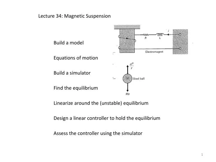
Lecture 34: Magnetic Suspension. Build a model. Equations of motion. Build a simulator. Find the equilibrium. Linearize around the (unstable) equilibrium. Design a linear controller to hold the equilibrium. Assess the controller using the simulator. Let me talk about the model.

E N D
Lecture 34: Magnetic Suspension Build a model Equations of motion Build a simulator Find the equilibrium Linearize around the (unstable) equilibrium Design a linear controller to hold the equilibrium Assess the controller using the simulator
Let me talk about the model Assume that the ball can only go up and down Gravity will pull the ball down: force mg down The magnet will pull the ball up: force needs discussion
I got this from another control book Let’s see what it says From Kuo BC Automatic Control Systems Kuo assumes an inverse relation, which is almost certainly wrong yis positive down Numerical parameters for later
What happens, more or less, is that the magnetic field magnetizes the ball turning it into a magnet pointing in the same direction as the coil magnet so we have N to S attraction The behavior depends on the geometry of the ball and its magnetic properties. There’s no attraction if the ball is not ferromagnetic
The coefficient c includes geometry, number of turns of the wire, permeability, etc There are many models of the force vs. gap equation none of them goes like 1/y I’ll talk about them shortly (and briefly) They are all inverse laws, and I can write where we need to think about the best value of n.
Different inverse models (different values of n) will have different constants An inverse square law (n = 2) is not a bad approximation, although there’s a wonderful quote I want to share “The only use, in fact, of the law of inverse squares, with respect to electromagnetism, is to enable you to write an answer when you want to pass an academical examination, set by some fossil examiner, who learned it years ago at the University, and never tried an experiment in his life to see if it was applicable to an electromagnet.” Thompson SP (1891) Lectures on the electromagnet WJ Johnson Co: NY All models agree that the force is proportional to the square of the B field which means to the square of the current, so that part of it is right
We can discuss the physical behavior qualitatively without settling the question as to the y dependence The magnetic force acts up and the gravity force acts down Whatever the model, the magnetic force decreases with distance and the gravity force is constant at mg There must be a distance where the two forces balance This is an equilibrium, but, as we can work out intuitively (and mathematically) it is NOT a stable equilibrium The next slide shows a schematic picture
Consider the stability from a physical perspective If the ball moves up the force increases and the ball accelerates up If the ball moves down the force decreases and the ball accelerates down
A brief survey of force models Analytic approximations for a pair of cylindrical magnets (from an old, old text from my undergraduate days) which we can scale
We can plot the variable part — the difference between this formula and 1/x2 is pretty small
Alternate theory: (Castañer R, Medina JM & Cuesta-Bolao MJ (2006) The magnetic dipole interaction as measured by spring dynamometers Am J Phys74 510-513.) which is verified by experiment, and suggests that n = 4 would be good
As it happens, the behavior of the system, and its control, is qualitatively the same the same for any of the inverse models I will choose inverse square despite the cruel words I quoted earlier, and I will use the numerical coefficients given in Kuo (slide 2)
What’s different about this problem from what we have done so far? We are going to have to linearize around a point other than zero We have a more complicated “Ohm’s Law” And we have our first state space with an odd number of dimensions — a third order problem
Manipulate the equations to build the state space picture combine these input
State vector We’ve added the current to the mechanical variables We can use these equations to set up our simulation We can integrate these equations numerically, using Mathematica, to simulate the system, but first let’s look at equilibrium
Equilibrium requires all the time derivatives to be zero From which we can express everything in terms of the equilibrium spacing
We can now set up the simulation and see how the equilibrium works We’ve argued on physical grounds that it is unstable, and we’ll argue later that it is unstable on mathematical grounds We make a simulation based on integrating the full equations of motion We denote the right hand side of the equations of motion by f + be
I’ve written f + be = F in the Mathematica I split the input e put in formal time dependence put in the numerical values of the parameters
Set up for an actual numerical integration this is an uncontrolled case The system is unstable, as we will see shortly, and after some time numerical round-off error functions as a perturbation and triggers exponential growth
We can look at that just before it happens by the time t = 2.04 it has blown up exponentially
We have a simulation, so now we can move on to control design The equations are nonlinear, so we need to linearize to deal with control To do that we use the equilibrium solution, which I found before
We want to linearize around the equilibrium solution This is the term that needs work I’ll deal with it on the next couple of slides
The linear equations We can make a matrix equation out of this
Let me note that there is another way to linearize this will seem weird to you, but it is very helpful once you believe it go back to the original nonlinear system Think of expanding f in a three variable Taylor series around the equilibrium
Remember that So that the expressions become And these are the columns of the linearized matrix We get b by differentiating the full equations with respect to e
This is really easy in Mathematica substitute the equilibrium condition
We have converted the original problem into a linear problem and we have converted our goal into making x go to zero The eigenvalues of A are We see that the system is unstable which anyone who’s ever tried to do this will know
Now we want to convert the linear problem to companion form (and make sure it is controllable) so it’s controllable Of course you can tell that it is of rank three by inspection
We want to use a gain matrix to stabilize this and then use to put it into the simulation
We want the departure from equilibrium to vanish and we want to place poles such that this is the case We have two negative roots of the undisturbed problem and one positive root
There is a set of poles often used in control problems: the Butterworth poles Butterworth, S (1930) “On the theory of filter amplifiers” Exptl Wireless and Wireless Engr Oct 1930 536-542. They lie equally-spaced on a circle in the left half plane Here are the Butterworth poles for a third order system
What happens if we simply move the positive root to -1? original poles controlled poles: move only the positive pole to -1 move the two close poles to 0.707 ± j 0.707
I have done extensive numerical experimentation and we can do more ourselves if we wish Butterworth poles work, but only if the radius is much bigger than 1 the nonlinearity interferes otherwise About the smallest I’ve been able to get to work is R = 43 but at that value it works quite well, and the control effort is not outrageous The larger the radius, the bigger the gains
We can look at the gains in x space as a function of the Butterworth radius At R = 43, the x gains are {30.3434, 1.02744, -2.03802}
The behavior of the system starting from rest at y = 0.45 y0 = 0.5 and the radius = 3
The behavior of the system starting from rest at y = 0.55 y0 = 0.5 and the radius = 3