Download
1 / 46
460 likes | 673 Vues
Queues. CSE, POSTECH. Queues. Like a stack, special kind of linear list One end is called front Other end is called rear Additions (insertions or enqueue) are done at the rear only Removals (deletions or dequeue) are made from the front only. Bus Stop. Bus Stop Queue.

E N D
Queues CSE, POSTECH
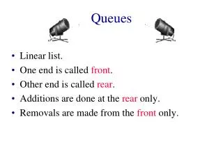
Queues • Like a stack, special kind of linear list • One end is called front • Other end is called rear • Additions (insertions or enqueue) are done at the rear only • Removals (deletions or dequeue) are made from the front only
Bus Stop Bus Stop Queue • Remove a person from the queue front rear rear rear rear rear
Bus Stop Bus Stop Queue front rear rear rear
Bus Stop Bus Stop Queue front rear rear
Bus Stop Bus Stop Queue • Add a person to the queue • A queue is a FIFO (First-In, First-Out) list. front rear rear
Queue ADT AbstractDataType queue { instances ordered list of elements; one end is the front; the other is the rear; operations empty(): Return true if queue is empty, return false otherwise size(): Return the number of elements in the queue front(): Return the front element of queue back(): Return the back (rear) element of queue pop(): Remove an element from the queue // dequeue push(x): Add element x to the queue // enqueue } It is also possible to represent Queues using Array-based representation Linked representation
The Abstract Class queue template <class T> // Program 9.1 class queue { public: virtual ~queue() {} virtual bool empty() const = 0; virtual int size() const = 0; virtual T& front() = 0; virtual T& back() = 0; virtual void pop() = 0; virtual void push(const T& theElement) = 0; };
Array-based Representation of Queue • Using simple formula equation location(i) = i – 1 • The first element is in queue[0], the second element is in queue[1], and so on • Front always equals zero, back (rear) is the location of the last element, and the queue sizeis rear + 1 • How much time does it need for pop()?
Derive from ArrayLinearList • When front is left end of list and rear is right end: • Queue.empty() ArrayLinearList.empty() O(1) • x = Queue.front() ArrayLinearList.get(0) O(1) • x = Queue.back() ArrayLinearList.get(length) O(1) • Queue.push(x) ArrayLinearList.insert(length, x) O(1) • Queue.pop() ArrayLinearList.erase(0) O(length) • To perform every operation in O(1) time, we need a customized array representation
Array-based Representation of Queue • Using modified formula equation location(i) = location(1) + i - 1 • No need to shift the queue one position left each time an element is deleted from the queue • Instead, each deletion causes front to move right by 1 • Front = location(1), rear = location(last element), and empty queue has rear < front • What do we do when rear = Maxsize –1 and front > 0?
Shifting a Queue Array-based Representation of Queue • Shifting a queue • To continue adding to the queue, we shift all elements to the left end of the queue • But shifting increases the worst-case add time from Q(1) to Q(n) Need a better method!
Array-based Representation of Queue • Remedy in modified formula equation that can provide the worst-case add and delete times in Q(1): location(i) = (location(1) + i – 1) % Maxsize • This is called a Circular Queue
Custom Array Queue • Use a 1D array queue • Circular view of array
Custom Array Queue • Possible configurations with three elements.
Custom Array Queue • Use integer variables ‘front’ and ‘rear’. • ‘front’ is one position counter-clockwise from first element • ‘rear’ gives the position of last element rear front
Custom Array Queue • Add an element • Move ‘rear’ one clockwise. • Then put an element into queue[rear].
Custom Array Queue • Remove an element • Move front one clockwise. • Then extract from queue[front].
Custom Array Queue • Moving clockwise • rear++; if (rear == queue.length) rear = 0; • rear = (rear + 1) % queue.length;
rear rear front front Custom Array Queue • Empty that queue
rear rear front front Custom Array Queue • Empty that queue
Custom Array Queue • Empty that queue • When a series of removals causes the queue to become empty, front = rear. • When a queue is constructed, it is empty. • So initialize front = rear = 0.
rear rear front front Custom Array Queue • A Full Tank Please
rear front rear front Custom Array Queue • A Full Tank Please
Custom Array Queue • A Full Tank Please • When a series of adds causes the queue to become full, front = rear. • So we cannot distinguish between a full queue and an empty queue. • How to differentiate two cases: queue empty and queue full?
Custom Array Queue • Remedies • Don’t let the queue get full • When the addition of an element will cause the queue to be full, increase array size • Define a boolean variable lastOperationIsAdd • Following each add operation set this variable to true. • Following each delete operation set this variable to false. • Queue is empty iff (front == rear) && !lastOpeartionIsAdd • Queue is full iff (front == rear) && lastOperationIsAdd
Custom Array Queue • Remedies (cont’d) • Define a variable NumElements • Following each add operation, increment this variable • Following each delete operation, decrement this variable • Queue is empty iff (front == rear) && (!NumElements) • Queue is full iff (front == rear) && (NumElements) • See Programs 9.2, 9.3, 9.4 • See Figure 9.7 for doubling array queue length
Linked Representation of Queue • Can represent a queue using a chain • Need two variables, front and rear, to keep track of the two ends of a queue • Two options: • assign head as front and tail as rear (see Fig 9.8 (a)), or • assign head as rear and tail as front (see Fig 9.8 (b)) Which option is better and why? See Figures 9.9 and 9.10
Head Tail Head Tail Figure 9.8 Linked Queues Linked Queue Representations
Add to & Delete from a Linked Queue • What is the time complexity for Fig 9.8 (a)? Θ(1) • What is the time complexity for Fig 9.8 (b)? Θ(1) • What is the time complexity for Fig 9.9 (a)? Θ(1) • What is the time complexity for Fig 9.9 (b)? Θ(n) • So, which option is better? Option 1
Linked Representation of Queue • How can we implement a linked representation of queue? • See Program 9.5 for implementing the push and pop methods of linkedQueue
lastNode firstNode NULL a b c d e front rear Derive From ExtendedChain • When front is left end of list and rear is right end: • empty() extendedChain::empty() • size() extendedChain::size() • front() get (0) • back() getLast() … new method • push(theElement) push_back(theElement) • pop() erase(0)
Revisit of Stack Applications • Applications in which the stack cannot be replaced with a queue • Parentheses matching • Towers of Hanoi • Switchbox routing • Method invocation and return • Application in which the stack may be replaced with a queue • Railroad Car Rearrangement • Rat in a maze
Application: Rearranging Railroad Cars • Similar to problem of Section 8.5.3 using stacks • This time holding tracks lie between the input and output tracks with the following same conditions: • Moving a car from a holding track to the input track or from the output track to a holding track is forbidden • These tracks operate in a FIFO manner can implement using queues • We reserve track Hk for moving cars from the input track to the output track. So the number of tracks available to hold cars is k-1.
Rearranging Railroad Cars • When a car is to be moved to a holding track, use the following selection method: • Move a car c to a holding track that contains only cars with a smaller label • If multiple such tracks exist, select one with the largest label at its left end • Otherwise, select an empty track (if one remains) • What happens if no feasible holding track exists? rearranging railroad cars is NOT possible • See Figure 9.11 and read its description
Implementing Rearranging Railroad Cars • What should be changed in previous program (in Section 8.5.3)? • Decrease the number of tracks (k) by 1 • Change the type of track to arrayQueue • What is the time complexity of rearrangement? • O(numberOfCars * k) • See Programs 9.6 and 9.7
Figure 9.12 Wire Routing Example Application: Wire Routing • Similar to Rat in a Maze problem in Section 8.5.6, but this time it has to find the shortest path between two points to minimize signal delay • Used in designing electrical circuit boards • Read the problem description on pg. 336
Wire Routing Algorithm The shortest path between grid positions a and b is found in two passes • Distance-labeling pass (i.e., labeling grids) • Path-identification pass (i.e., finding the shortest path)
Figure 9.13 Wire Routing Wire Routing Algorithm 1. Labeling Grids: Starting from position a, label its reachable neighbors 1. Next, the reachable neighbors of squares labeled 1 are labeled 2. This labeling process continues until we either reach b or have no more reachable squares. The shaded squares are blocked squares.
Figure 9.13 Wire Routing Wire Routing Algorithm 2. Finding the shortest path: Starting from position b, move to any one of its neighbors labeled one less than b’s label. Such a neighbor must exist as each grid’s label is one more than that of at least one of its neighbors. From here, we move to one of its neighbors whose label is one less, and so on until we reach a.
Wire Routing Algorithm Exercise Consider the wire-routing grid of Figure 9.13(a). You are to route a wire between a=(1, 1) and b=(1, 6). Label all grid positions that are reached in the distance-labeling pass by their distance value. Then use the methodology of the path-identification pass to mark the shortest wire path. Is there only one shortest path?
Implementing Wire Routing Algorithm • An m x m grid is represented as a 2-D array with a 0 representing an open position and a 1 representing a blocked position • the grid is surrounded by a wall of 1s • the array offsets helps us move from a position to its neighbors • A queue keeps track of labeled grid positions whose neighbors have yet to be labeled • What is the time complexity of the algorithm? O(m2) for labeling grids & O(length of the shortest path) for path construction • Read Program 9.8
Application: Image-Component Labeling • Background information: • A digitized image is an m x m matrix of pixels. • In a binary image, each pixel is 0 or 1. • A 0 pixel represents image background, while a 1 represents a point on an image component. • Two pixels are adjacent if one is to the left, above, right, or below the other. • Two component pixels that are adjacent are pixels of the same image component. • Problem: Label the component pixels so two pixels get the same label iff they are pixels of the same image component.
Figure 9.14 Image-Component Labeling Image-Component Labeling Example • The blank squares represent background pixels and 1s represent component pixels • Pixels (1,3), (2,3), and (2,4) are from the same component
Image-Component Labeling Algorithm • Idea:Similar to the wire-routing problem • Steps: • Scan pixels one by one (row-major search). • When encounter a 1 pixel, give a unique component identifier. • Find all neighbors by expanding from that pixel and give the unique identifier. • Repeat for all pixels. • See program 9.9 • What is the time complexity of Program 9.9?
READING • Read 9.5.4 Machine Shop Simulation • Read all of Chapter 9