Download
1 / 43
430 likes | 633 Vues
The Ocean-Land-Atmosphere Model (OLAM) Robert L. Walko Roni Avissar Rosenstiel School of Marine and Atmospheric Science University of Miami, Miami, FL Martin Otte U.S. Environmental Protection Agency Research Triangle Park, NC 27711 David Medvigy

E N D
The Ocean-Land-Atmosphere Model (OLAM) Robert L. Walko Roni Avissar Rosenstiel School of Marine and Atmospheric Science University of Miami, Miami, FL Martin Otte U.S. Environmental Protection Agency Research Triangle Park, NC 27711 David Medvigy Department of Geosciences and Program in Atmospheric and Oceanic Sciences, Princeton University, Princeton, NJ
External GCM domain RAMS domain Information flow Numerical noise at lateral boundary OLAM global lower resolution domain OLAM local high resolution region Information flow Well behaved transition region Motivation for OLAM originated in our work with the Regional Atmospheric Modeling System (RAMS) RAMS, begun in 1986, is a limited-area model similar to WRF and MM5 Features include 2-way interactive grid nesting, microphysics and other physics parameterizations designed for mesoscale & microscale simulations But, there are significant disadvantages to limited-area models So, OLAM was originally planned as a global version of RAMS. OLAM began with all of RAMS’ physics parameterizations in place.
Global RAMS 1997: “Chimera Grid” approach Lateral boundary values interpolated from interior of opposite grid Not flux conservative
OLAM dynamic core is a complete replacement from RAMS Seamless local mesh refinement Based on icosahedral grid
OLAM: Relationship between triangular and hexagonal cells (either choice uses Arakawa-C grid stagger)
OLAM: Hexagonal grid cells
Downscaling Regional Climate Model Simulations to the Spatial Scale of the Observations
Terrain-following coordinates used in most models OLAM uses cut cell method
One reason to avoid terrain-following grids: Error in horizontal gradient computation (especially for pressure) P P V V P P
Wind Another reason: Anomalous vertical dispersion Thin cloud layer Terrain-following coordinate levels Terrain
Continuous equations in conservation form Momentum conservation (component i) Total mass conservation conservation Equation of State Scalar conservation (e.g. ) Total density Momentum density = potential temperature = ice-liquid potential temperature
Finite-volume formulation: Integrate over finite volumes and apply Gauss Divergence Theorem , Discretized equations: .
Conservation equations in discretized finite-volume form (SGS = “subgrid-scale eddy correlation”) cell volume cell face area Discretized momentum density is consistent between all conservation equations
Grid cells A and B have reduced volume and surface areaFully-underground cells have zero surface area A B
Land cells are defined such that each one interacts with only a single atmospheric level Land grid cells
Cut cells vs. terrain-following coordinates • High vertical resolution near ground • Direction of atmospheric isolines
C-staggered momentum advection method of Perot (JCP 2002) 3D wind vector diagnosed Normal wind prognosed
Neighbors of W point on hexagonal mesh itab_w(iw)%im(1:7) itab_w(iw)%iv(1:7) itab_w(iw)%iw(1:7) iw5 iw4 iv5 im4 iv4 im5 iw6 iv6 im3 im6 iw iv3 iw3 im2 iv7 iw7 im7 iv2 im1 iv1 iw2 iw1
Neighbors of V point on hexagonal mesh itab_v(iv)%im(1:6) itab_v(iv)%iv(1:16) itab_v(iv)%iw(1:4) iw4 iv11 iv10 im6 im5 iv12 iv9 iv3 iv4 im2 iv15 iv16 iv iw1 iw2 iu iv14 im1 iv13 iv2 iv5 iv8 iv1 im4 im3 iw3 iv6 iv7
Neighbors of M point on hexagonal mesh itab_m(im)%iv(1:3) itab_m(im)%iw(1:3) iv3 iw1 iw2 im iv2 iv1 iw3
RAMS/OLAM Bulk Microphysics Parameterization • Physics based scheme – emphasizes individual microphysical processes rather than the statistical end result of atmospheric systems • Intended to apply universally to any atmospheric system (e.g., convective or stratiform clouds, tropical or arctic clouds, etc.) • Represents microphysical processes that are considered most important for most modeling applications • Designed to be computationally efficient
Physical Processes Represented • Cloud droplet nucleation • Ice nucleation • Vapor diffusional growth • Evaporation/sublimation • Heat diffusion • Freezing/melting • Shedding • Sedimentation • Collisions between hydrometeors • Secondary ice production
Hydrometeor Types • Cloud droplets • Drizzle • Rain • Pristine ice (crystals) • Snow • Aggregates • Graupel • Hail C D R P S A G H
Stochastic Collection Equation Table Lookup Form of Collection Equation
A wav hav was has wca hca wca hca hvc hvc wvc wvc rvc rav C V V wvs hvs LEAF–4 fluxes C rsv wsc hsc rsa S2 S1 wss hss longwave radiation sensible heat water rga wgvc2 rgv wgc hgc G2 wgs hgs wgvc2 G2 wgvc1 wgvc1 wgg hgg wgg G1 hgg G1 LANDCELL 1 LANDCELL 2
Water flux between soil layers Hydraulic conductivity(m/s) Soil water potential (m) Ks = saturation hydraulic conductivity ys = saturation water potential rw = density of water [h/ hs] = soil moisture fraction b = 4.05, 5.39, 11.4 for sand, loam, clay
How should models represent convection at different grid resolutions? Conventional thinking is to resolve convection where possible and to parameterize it otherwise. ? Deep Convection resolve parameterize Shallow Convection ? resolve parameterize 0.1 1 10 100 Horizontal grid spacing (km)