Download
1 / 15
150 likes | 332 Vues
Electron poor materials research group. Group meeting Nov 11, 2010 Theory- Bader Analysis -> FCC This is version 2 with larger NG(X,Y,Z)F values for more accurate charge density grids. Pre-Procedure.

E N D
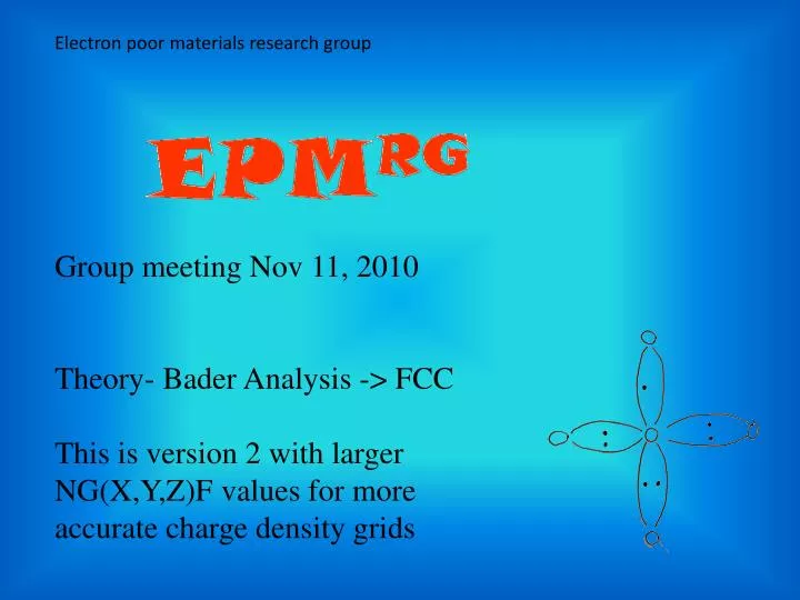
Electron poor materials research group Group meeting Nov 11, 2010 Theory- Bader Analysis -> FCC This is version 2 with larger NG(X,Y,Z)F values for more accurate charge density grids
Pre-Procedure • Very accurate Equation of state (EOS) calculations are preformed to find the optimum relaxed volume of the structure. This EOS is fitted to a Birch-Murnaghan equation. • 11X11X11 kpoint gamma grid • PREC=ACCURATE • ENCUT=1.3*(ENMAX in POTCAR) • Psuedo-potential is PAW_PBE • A final very accurate final relaxation if preformed to bring the structures to their final relaxation volume given by EOS • see next slide for INCAR for relaxation
INCAR for final relaxation System = Si relaxsetup.sh NSW = 20 | number of ionic steps ISIF = 4 | (ISIF=2 Relax ions only, ISIF=3 Relax everything) IBRION = 1 | ionic relaxation algorithm EDIFF = 1E-9 | break condition for elec. SCF loop EDIFFG = -1E-8 | break condition for ionic relaxation loop MAXMIX = 80 | keep dielectric function between ionic movements NELMIN = 8 | minimum number of electronic steps NFREE = 20 | number of degrees of freedom (don't go above 20) #RECOMMENDED MINIMUM SETUP #GGA= #xchange-correlation #VOSKOWN= #=1 if GGA=91; else = 0 PREC = ACCURATE #PRECISION, sets fft grid ENCUT = 320 #energy cutoff, determines number of lattice vectors LREAL = .FALSE. #.FALSE. MEANS USE RECIPROCAL LATTICE ISMEAR = 0 #determines how partial occupancies a set.
Procedure • Static Calculations of the 4 FCC structures were computed from accurate relaxation (see previous slides) • Calculations were done on a Gamma 11X11X11 grid • USED NG(X,Y,Z)F of 6XNG(X,Y,Z) for accurate charge density grid. • An extra flag was used in the INCAR file: LAECHG = .TRUE. • Turns on All Electron CHGCAR file outputs and outputs 3 files • AECCAR0: core charge density • AECCAR1: atomic AE charge density (overlapping atomic charge density) • AECCAR2: AE charge density • The files AECCAR0 and AECCAR2 are added together for bader analysis per instructions: http://theory.cm.utexas.edu/bader/vasp.php • chgsum.sh AECCAR0 AECCAR2, chsum is a shellscript • Outputs CHGCAR_sum • Bader analysis is done on the vasp CHGCAR from the static run • bader.x -p atom_index -p bader_index CHGCAR -ref CHGCAR_sum • atom_index: Write the atomic volume index to a charge density file • bader_index: Write the Bader volume index to a charge density file
NOTES • Only the PAW potentials can output there core charges for bader analysis • A fine fft grid is needed to accurately reproduce the correct total core charge. It is essential to do a few calculations, increasing NG(X,Y,Z)F until the total charge is correct. • The outputs from bader.x are: • ACF.dat – Atomic Coordinate file. Shows the location and charge of the atoms • BCF.dat – Bader Coordinate file. • AVF.dat – Atomic Volume file. Used to keep track of other files that may be output with the bader program with flag –p all_atom • AtIndex.dat (only with –p atom_index) – charge density file which contains the atomic borders • BvIndex.dat (only with –p bader_index) –charge density file which contains the bader borders
INCAR_static System = Si SIGMA = 0.01 #RECOMMENDED MINIMUM SETUP PREC = ACCURATE #PRECISION ENCUT = 320 LREAL = .FALSE. #.FALSE. MEANS USE RECIPROCAL LATTICE ISMEAR = 0 #USE GAUSSIAN SMEARING #FOR GW CALCULATIONS #LOPTICS = .TRUE. #NBANDS = 96 #FOR BADER ANALYSIS LAECHG=.TRUE. NGXF = 120 #USE 6X NGX for bader analysis NGYF = 120 NGZF = 120 .
GaAs ACF.dat : # X Y Z CHARGE MIN DIST ATOMIC VOL -------------------------------------------------------------------------------- 1 0.0000 0.0000 0.0000 2.3763 1.0539 18.1315 2 1.4409 1.4409 1.4409 5.6237 1.2766 29.7299 -------------------------------------------------------------------------------- VACUUM CHARGE: 0.0000 VACUUM VOLUME: 0.0000 NUMBER OF ELECTRONS: 8.0000 ENAs – ENGa = 0.37 Bader charge shift = 0.6237
GaAs Bader Volume Bounding Boxes All other FCC bounding boxes look virtually identical to this one
InSb ACF.dat : # X Y Z CHARGE MIN DIST ATOMIC VOL -------------------------------------------------------------------------------- 1 0.0000 0.0000 0.0000 2.6001 1.2796 29.8830 2 1.6622 1.6622 1.6622 5.3999 1.4473 43.5992 -------------------------------------------------------------------------------- VACUUM CHARGE: 0.0000 VACUUM VOLUME: 0.0000 NUMBER OF ELECTRONS: 8.0000 ENSb – ENIn = 0.27 Bader charge shift = 0.3999
GaSb ACF.dat : # X Y Z CHARGE MIN DIST ATOMIC VOL -------------------------------------------------------------------------------- 1 0.0000 0.0000 0.0000 2.7022 1.1483 22.2941 2 1.5563 1.5563 1.5563 5.2978 1.4227 38.0197 -------------------------------------------------------------------------------- VACUUM CHARGE: 0.0000 VACUUM VOLUME: 0.0000 NUMBER OF ELECTRONS: 8.0000 ENSb – ENGa = 0.24 Bader charge shift = 0.2978
ZnSe ACF.dat : # X Y Z CHARGE MIN DIST ATOMIC VOL -------------------------------------------------------------------------------- 1 0.0000 0.0000 0.0000 11.2714 1.0616 15.9986 2 1.4358 1.4358 1.4358 6.7286 1.3224 31.3555 -------------------------------------------------------------------------------- VACUUM CHARGE: 0.0000 VACUUM VOLUME: 0.0000 NUMBER OF ELECTRONS: 18.0000 ENSe – ENZn = 0.9 Bader charge shift = 0.7286
ZnTe ACF.dat : # X Y Z CHARGE MIN DIST ATOMIC VOL -------------------------------------------------------------------------------- 1 0.0000 0.0000 0.0000 11.4898 1.1104 18.5303 2 1.5464 1.5464 1.5464 6.5102 1.4456 40.6387 -------------------------------------------------------------------------------- VACUUM CHARGE: 0.0000 VACUUM VOLUME: 0.0000 NUMBER OF ELECTRONS: 18.0000 ENTe – ENZn = 0.45 Bader charge shift = 0.5102
Si - For Comparison ACF.dat : # X Y Z CHARGE MIN DIST ATOMIC VOL -------------------------------------------------------------------------------- 1 0.0000 0.0000 0.0000 3.9681 1.1316 20.2891 2 1.3672 1.3672 1.3672 4.0319 1.1051 20.6007 -------------------------------------------------------------------------------- VACUUM CHARGE: 0.0000 VACUUM VOLUME: 0.0000 NUMBER OF ELECTRONS: 8.0000 ENTe – ENZn = 0.0 Bader charge shift = 0.0319