Download
1 / 33
330 likes | 402 Vues
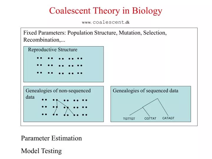
Coalescent Theory in Biology www. coalescent .dk. Fixed Parameters: Population Structure, Mutation, Selection, Recombination,. Reproductive Structure. Genealogies of non-sequenced data. Genealogies of sequenced data. CATAGT. CGTTAT. TGTTGT. Parameter Estimation Model Testing.

E N D
Coalescent Theory in Biology www. coalescent.dk Fixed Parameters: Population Structure, Mutation, Selection, Recombination,... Reproductive Structure Genealogies of non-sequenced data Genealogies of sequenced data CATAGT CGTTAT TGTTGT Parameter Estimation Model Testing
Wright-Fisher Model of Population Reproduction Haploid Model i. Individuals are made by sampling with replacement in the previous generation. ii. The probability that 2 alleles have same ancestor in previous generation is 1/2N Assumptions Constant population size No geography No Selection No recombination Diploid Model Individuals are made by sampling a chromosome from the female and one from the male previous generation with replacement
P(k):=P{k alleles had k distinct parents} 1 1 2N Ancestor choices: k -> k k -> any k -> k-1 k -> j (2N)k 2N *(2N-1) *..* (2N-(k-1)) =: (2N)[k] Sk,j - the number of ways to group k labelled objects into j groups.(Stirling Numbers of second kind. For k << 2N:
Waiting for most recent common ancestor - MRCA Distribution until 2 alleles had a common ancestor, X2?: P(X2 > j) = (1-(1/2N))j P(X2 > 1) = (2N-1)/2N = 1-(1/2N) P(X2 = j) = (1-(1/2N))j-1 (1/2N) j j 2 2 1 1 1 1 1 1 2N 2N 2N Mean, E(X2) = 2N. Ex.: 2N = 20.000, Generation time 30 years, E(X2) = 600000 years.
Multiple and Simultaneous Coalescents 1. Simultaneous Events 2. Multifurcations. 3. Underestimation of Coalescent Rates
Discrete Continuous Time tc:=td/2Ne 6 6/2Ne 0 2N 0 1 4 1.0 corresponds to 2N generations 1.0 0.0 2 6 5 3
1 2 3 4 5 The Standard Coalescent Two independent Processes Continuous: Exponential Waiting Times Discrete: Choosing Pairs to Coalesce. Waiting Coalescing {1,2,3,4,5} (1,2)--(3,(4,5)) {1,2}{3,4,5} 1--2 {1}{2}{3,4,5} 3--(4,5) {1}{2}{3}{4,5} 4--5 {1}{2}{3}{4}{5}
Expected Height and Total Branch Length Branch Lengths Time Epoch 1 2 1 2 1 1/3 3 2/(k-1) k Expected Total height of tree: Hk= 2(1-1/k) i.Infinitely many alleles finds 1 allele in finite time. ii. In takes less than twice as long for k alleles to find 1 ancestors as it does for 2 alleles. Expected Total branch length in tree, Lk: 2*(1 + 1/2 + 1/3 +..+ 1/(k-1)) ca= 2*ln(k-1)
Effective Populations Size, Ne. In an idealised Wright-Fisher model: i. loss of variation per generation is 1-1/(2N). ii. Waiting time for random alleles to find a common ancestor is 2N. Factors that influences Ne: i.Variance in offspring. WF: 1. If variance is higher, then effective population size is smaller. ii.Population size variation - example k cycle: N1, N2,..,Nk. k/Ne= 1/N1+..+ 1/Nk. N1 = 10 N2= 1000 => Ne= 50.5 iii.Two sexesNe = 4NfNm/(Nf+Nm)I.e. Nf-10Nm -1000 Ne - 40
6 Realisations with 25 leaves Observations: Variation great close to root. Trees are unbalanced.
Sampling more sequences The probability that the ancestor of the sample of size n is in a sub-sample of size k is Letting n go to infinity gives (k-1)/(k+1), i.e. even for quite small samples it is quite large.
Adding Mutations m mutation pr. nucleotide pr.generation. L: seq. length µ = m*L Mutation pr. allele pr.generation. 2Ne - allele number. Q := 4N*µ -- Mutation intensity in scaled process. Continuous time Continuous sequence Discrete time Discrete sequence 1/L time 1/(2Ne) time sequence sequence mutation mutation coalescence Probability for two genes being identical: P(Coalescence < Mutation) = 1/(1+Q). 1 Q/2 Q/2 Note: Mutation rate and population size usually appear together as a product, making separate estimation difficult.
Three Models of Alleles and Mutations. Finite Site Infinite Allele Infinite Site acgtgctt acgtgcgt acctgcat tcctgcat tcctgcat Q Q Q acgtgctt acgtgcgt acctgcat tcctggct tcctgcat i. Allele is represented by a sequence. ii. A mutation changes nucleotide at chosen position. i. Only identity, non-identity is determinable ii. A mutation creates a new type. i. Allele is represented by a line. ii. A mutation always hits a new position.
Infinite Allele Model 4 5 1 2 3
Infinite Site Model Final Aligned Data Set:
Labelling and unlabelling:positions and sequences 1 2 3 4 5 Ignoring mutation position Ignoring sequence label 1 2 3 5 4 Ignoring mutation position Ignoring sequence label { , , } The forward-backward argument 4 classes of mutation events incompatible with data 9 coalescence events incompatible with data
Infinite Site Model: An example Theta=2.12 2 3 2 3 4 5 5 9 5 10 14 19 33
Finite Site Model acgtgctt acgtgcgt acctgcat tcctgcat tcctgcat s s s Final Aligned Data Set:
Diploid Model with Recombination An individual is made by: The paternal chromosome is taken by picking random father. Making that father’s chromosomes recombine to create the individuals paternal chromosome. Similarly for maternal chromosome.
The Diploid Model Back in Time. A recombinant sequence will have have two different ancestor sequences in the grandparent.
1- recombination histories I:Branch length change 1 2 4 3 2 1 4 3 2 1 4 3
1- recombination histories II:Topology change 1 2 4 3 2 1 4 3 2 1 4 3
1- recombination histories III:Same tree 1 2 4 3 2 1 4 3 2 1 4 3
1- recombination histories IV:Coalescent time must be further back in time than recombination time. c r 1 2 4 3
Recombination-Coalescence Illustration Copied from Hudson 1991 Intensities Coales.Recomb. 0 1 (1+b) b 3 (2+b) 6 2 3 2 1 2
From Wiuf and Hein, 1999 Genetics Age to oldest most recent common ancestor Scaled recombination rate - r 0 kb 250 kb Age to oldest most recent common ancestor
Number of genetic ancestors to the Human Genome Sr– number of Segments E(Sr) = 1 + r time C C C R R R sequence Simulations Statements about number of ancestors are much harder to make.
Applications to Human Genome (Wiuf and Hein,97) 0 260 Mb 0 52.000 *35 0 7.5 Mb 6890 8360 *250 30kb 0 Parameters used 4Ne 20.000 Chromos. 1: 263 Mb. 263 cM Chromosome 1: Segments 52.000 Ancestors 6.800 All chromosomes Ancestors 86.000 Physical Population. 1.3-5.0 Mill. A randomly picked ancestor: (ancestral material comes in batteries!)
1 2 3 4 1 2 4 3 Ignoring recombination in phylogenetic analysis General Practice in Analysis of Viral Evolution!!! Recombination Assuming No Recombination Mimics decelerations/accelerations of evolutionary rates. No & Infinite recombination implies molecular clock.
Genotype and Phenotype Covariation: Gene Mapping Decay of local dependency Time Reich et al. (2001) Genetype -->Phenotype Function Dominant/Recessive. Penetrance Spurious Occurrence Heterogeneity genotype phenotype Genotype Phenotype Sampling Genotypes and Phenotypes Result:The Mapping Function A set of characters. Binary decision (0,1). Quantitative Character.