Download
1 / 50
500 likes | 622 Vues
The Level-2 jet trigger and SUSY studies with the ATLAS detector. Ignacio Aracena University of Bern SLAC, Nov. 16 th 2006. Outline. Introduction Supersymmetry & mSUGRA The LHC and the ATLAS detector The ATLAS trigger system The Level-2 jet trigger SUSY decay chain

E N D
The Level-2 jet trigger and SUSY studies with the ATLAS detector Ignacio Aracena University of Bern SLAC, Nov. 16th 2006
Outline • Introduction • Supersymmetry & mSUGRA • The LHC and the ATLAS detector • The ATLAS trigger system • The Level-2 jet trigger • SUSY decay chain • SUSY events in the electron trigger • Summary I. Aracena
Introduction • Matter ↔ forces interactions are well described by the Standard Model (SM) • In the SM the “Higgs mechanism” generates the particles’ masses • No Higgs particle discovered yet. • SM has shortcomings. It is not the fundamental theory. • New physics phenomena expected at the TeV scale. • A very high luminosity particle accelerator colliding particles at the TeV energy scale is needed! • The Large Hadron Collider • Need an adequate detector to exploit the physics potential • The ATLAS detector I. Aracena
Motivation for Supersymmetry The naturalness problem: mHiggs ~ MPlanck? • Quadratically divergent correction to scalar mass • Corrections cancel (up to lnL) if for each fermion loop an associated boson loop exists No unification of the three forces in the SM? • Introduce new supersymmetric particles which yield unification of the gauge couplings at the GUT scale. 2 2 Introduce new symmetry between fermions and bosons: Supersymmetry! I. Aracena
Minimal Supersymmetric Standard Model • The “minimal” implementation of supersymmetry is called Minimal Supersymmetric (extention) of the SM (MSSM) • Solves naturalness problem, unification of couplings • Supersymmetry must be broken • Sparticles have not been seen so far Mslepton ≠ Mlepton (heavier than our current reach) • But don’t know how it is broken: • Several supersymmetry breaking scenarios (SUGRA,GMSB,...) • Each scenario leads to a different phenomenology • Depends on 105 free parameters • MSSM allows proton decay! • Introduce R=(−1)3B−3L−2S parity conservation • Ligthest SUSY Particle (LSP) is stable • If only weakly interacting a perfect candidate for cold dark matter I. Aracena
MSSM particles • After supersymmetry and electroweak symmetry breaking, sparticles mix • to form the physical mass eigenstates • Chargino sector: mixing of • Neutralino sector: mixing of • Large mixing in third generation squark and sleptons • Higgs sector: 5 physical states h, H, A, H± • Assume R-parity conservation: • Sparticles are produced in pairs. • The lightest supersymmetric particle (LSP) is stable • Assume LSP is electrically neutral and color-neutral • Interacts only weakly with ordinary matter invisible in the detector In pp- collider experiments: missing energy from two invisible LSPs in the final state! I. Aracena
mSUGRA • minimal Super Gravity postulates that hidden and visible sector communicate through gravity • A good framework for studies of SUSY searches at future colliders • Reduces the number of free parameters to five at the GUT scale: • m0 common scalar mass • m1/2 common fermion mass • tanb = vu/vd Higgs vacuum expectation values • A0 common trilinear coupling • sgn(m) sign of Higgs mass parameter • mSUGRA used for ATLAS studies with full detector simulation I. Aracena
Typically σ>1pb with sparticle masses <1TeV The LHC reach! ~ mSUGRA (m1/2,m0)-plane Different regions in the mSUGRA parameter space characterized according to the mechanims that leads to the observed WCDM Coannihilation region LSP-NLSP coannihilation Funnel region large tanb 2m(LSP)~m(H,A) Bulk region largely reduced by WMAP LSP-LSP annihilation trough slepton exchange Focus point region LSP higgsino-like I. Aracena
n n e e µ µ p p n n p-p collisions at the LHC Nominal LHC Parameters: 7 TeV Proton Energy 1034cm-2s-1 Luminosity 2808 Bunches per Beam 1011 Protons per Bunch 25ns 7.5m Bunch Crossings 4x10⁷ Hz Proton-Proton Collisions 109 Hz Quark/Gluon Collisions I. Aracena
Detector requirements In order to exploit the LHC physics potential, build a multipurpose detector with: • Very good calorimetry with good hermeticity • Efficient tracking for precision lepton momentum measurement • Precision muon momentum measurement with standalone capability • Fast trigger system • Radiation hard detector The ATLAS detector I. Aracena
p p The ATLAS detector Diameter 25 m Barrel toroid length 26 m End-cap end-wall chamber span 46 m Overall weight 7000 Tons AToroidal LHC ApparatuS I. Aracena
Physics events at the LHC Event rate at the LHC is 1GHz! Cannot record all events on tape, but: Minimum bias events, SM physics at ~MHz Reject uninteresting events online + Interesting new physics (SUSY) at ≤Hz rate! Select interesting events online = The ATLAS trigger system I. Aracena
The ATLAS trigger Level 1 (hardware): Defines Regions of Interest (RoI). Uses Calo cells and Muon chambers with reduced granularity. e/g, m, t, jet candidates. 2ms Execution time <75(100) kHz High Level Trigger (PC farm) 10ms Level 2 O(500PCs): Seeded by LVL1 RoI. Full granularity of the detector Performs calo-track matching ~2 kHz 1s ~200 Hz Event Filter O(1900PCs): Offline-like algorithms. Refines LVL2 decision Full event building TIER 0 mass storage I. Aracena
Trigger menu table 2e15i stands for at least two isolated electrons with pt>15GeV for both of them I. Aracena
The Level-2 jet trigger package • Uses Level-1 jet RoI as seed. • Calls a number of tools: • Data preparation tool: Access selected calo region around the Level-1 jet RoI. • Cone algorithm: Assume cone-shaped jet with defined Rcone. • Calibration: Calibrate jet energy using sampling technique. I. Aracena
The Level-2 jet data preparation The data preparation tool is the most critical in terms of timing performance (O(106) calorimeter cells) Two data preparation methods implemented: • T2CaloJetGridFromCells (cell jets): Uses full granularity of the ATLAS calorimeters. • T2CaloJetGridFromFEBHeader (LArFEB jets): Uses information from the LAr calorimeter Front End Boards (FEB). Uses cell-granularity for the tile calorimeter. One FEB receives signals from 128 calorimeter channels. Calculate Ex, Ey, Ez over all channels connected to one FEB. Translate this into ET, h, f . I. Aracena
Level-2 jet energy calibration Need to correct the energy scale: T2CaloJetCalibTool • Use sampling techniqueE(rec)=wem(η)E(em)+whad(η)E(had), • wem,had = a+blog(E) • Estimate weights by minimizing • Compute weights for bins in η with ∆η(bin)=0.1 • Weights obtained using cell-based method • Apply computed weights to cell- and LArFEB-jets I. Aracena
Level-2 trigger algorithm Half Width • A TrigT2Jet object is created with L1 h, f. • Data preparation tool access data around the L1 ROI (HalfWidth). Creates grid of detector readout elements (grid elements). • Jet Cone algorithm iteration (N times): • Set inCone flag for gridElements inside cone radiusRcone=(∆h2+ ∆f2)1/2 • Calculate energy-weighted h,f. • Updates TrigT2Jet e, h, f. • Iterate N times. • Apply calibration weights. • Export final values. ConeRadius ROI N iterations ROI Study jet trigger performance as a function of: Data preparation tool, RoI HalfWidth, N iterations, coneRadius, calibration weights. I. Aracena
L2 jet system performance Difference between two consecutive iterations of T2CaloJetConeTool (Using 1000 dijet events pt>2240GeV) ∆E=jetN(E)−jetN-1(E) ∆R=jetN(R)−jetN-1(R) T2CaloJetConeTool converges after 3-4 iterations (cell- and LArFEB-based) I. Aracena
L2 jet system performance Number of grid elements prepared by the data preparation tools LArFEB method reduces the amount of data by one order of magnitude. I. Aracena
L2 jet timing Level-2 jet timing performance (in ms, 2.8GHz) Map (h,f)-region to detector ID Convert bytestream to C++ objects for LAr and tile calo Prepare all grid elements inside cone One iteration of the cone algorithm LArFEB method reduces the amount of data by one order of magnitude. Significant impact on timing. I. Aracena
Physics performance Use QCD dijet samples: Compare L2 jets with MC truth jets: • Cone algorithm • Rcone=0.4, Eseed > 2GeV, Econe > 10GeV • Use Level-2 jet algorithm parameters: • cell- and LArFEB method, Rcone=0.4, RoI HalfWidth=0.7, N iterations=3 I. Aracena
L2 jet – position resolution Cell-jets LArFEB-jets σ=2.8 σ=3.0 Compatible position resolution for cell- and LArFEB-based methods. I. Aracena
L2 jet energy scale Data sample 70 < pT < 140 Cell-based LArFEB-based EL2/EMC~1 EL2/EMC>1 Larger spread Need dedicated LArFEB weights! I. Aracena
L2 jet energy scale Data sample 1120 < pT < 2240 Cell-based LArFEB-based EL2/EMC>1 Larger spread Need dedicated LArFEB weights! EL2/EMC~<1 Difference between detector layout I. Aracena
SUSY searches at ATLAS In the mSUGRA bulk region
ATLAS mSUGRA points Following points have been chosen for study with the full ATLAS detector simulation The results shown in this talk are in the bulk region I. Aracena
The bulk region Mass hierarchy mSUGRA Parameters: M0 = 100GeV M1/2 = 300GeV A0 = − 300GeV tanβ = 6 σLO = 19.3pb Long decay chains: large missing ET and high-pt jets +leptons in the final state The following results are obtained using this mSUGRA scenario and using the full ATLAS detector simulation. I. Aracena
Inclusive SUSY searches Typical SUSY event contains at least 4 jets+missing Et Effective mass missEt>max(0.2Meff,100GeV) 1,2 jets Pt>100GeV 3,4 jets Pt>50GeV Bulk region 4.20fb−1 I. Aracena
ATLAS Bulk region 4.20fb−1 p p • only SUSY signal (full sim.) • select events with 2 leptons Exclusive signatures • After initial discovery of SUSY the measurement of the sparticle masses will be the next step. • Two invisible LSP in each event, so no direct mass measurement possible. • Obtain kinematic edges from invariant mass distributions of involved particles, e.g. dilepton distribution mll. • Remove SUSY/SM BG using OppositeFlavor/OppositeSign (OF/OS) pairs, e.g. . I. Aracena
large small mllq (GeV) mllq (GeV) Leptons+jets distributions - mllq Obtain more edges: include the quark coming from the squark decay Combine the two leptons with the two hardest jets in the event: p p Bulk region: signal evts (full sim.); ≥2 jets and 2 leptons. Apply OF/OS subtraction. 16 12 8 4 0 60 50 40 30 20 10 0 ATLAS 4.20fb−1 ATLAS 4.20fb−1 Entries/10Gev Entries/10Gev full sim. full sim. 0 200 400 600 800 1000 0 200 400 600 800 1000 I. Aracena
MC truth (Herwig) Bulk region Tau signatures Decay chains involving taus are challenging, due to: • Escaping neutrino. • Only consider hadronic tau decays. Distorted shape of the ditau mass distribution. They are particularly interesting: • for large tanβ, decays into have large BR. • Can use tau polarization measurement to further constrain the underlying SUSY model. I. Aracena
Reconstruct the dilepton inv. mass in the decay chain. Shape of can be calculated given knowledge of tau polarizations. Extracting polarization is challenging. mττ (vis)/98.3 Ditau mass distribution • Bulk region • select events with two reconstructed taus. • Uncorrelated pairs accounted • for by using same-sign pairs. • True endpoint • Endpoint structure visible at the expected • value. ATLAS 4.2fb−1 full sim. mττ (vis) (GeV) Use MC truth as a first approx. and fit obtained function to data. I. Aracena
SUSY and trigger? • In the shown plots trigger effects are not taken into account, i.e. assume 100% trigger efficiency. • In the real experiment the trigger will select online the events. • Events rejected by the trigger are lost forever! • Need to understand and plan a concise strategy for triggering on SUSY events. trigger-aware analysis! I. Aracena
No. events after L1/L2/EF Eff = No. events with ≥1 e± in MC truth Electron trigger – e25i The Level-1 electron trigger • Electron trigger: • look for isolated EM cluster • match cluster to reconstructed track (only L2 & EF) hadronic isolation EM isolation Tune “e25i” trigger item with single electrons with ET=25GeV: central Region of Interest (RoI) cluster I. Aracena
Complex SUSY event signatures non-isolated electrons e25i trigger – with SUSY Estimate e25i trigger efficiency using SUSY sample Level1 EM25i cuts (GeV) tuned for 95% efficiency: ClusterET > 19 EmRingIsol < 3 HadIsol < 2 Remove isolation at LVL1: ClusterET > 19 EmRingIsol < 999999 HadIsol < 999999 I. Aracena
Electron efficiency – SUSY • How many good events are lost in the trigger (compared to offline)? • Compare pt distribution of leading electron (bulk+pileup 1033cm–2s–1): • offline reconstruction PT>15GeV, |h|<2.5 • offline reconstruction + electron trigger e25i||2e15i||e60 90% of the offline events (e25i||2e15i||e60) are also triggered I. Aracena
Summary • The Level-2 jet trigger implemented and running. • Choice between cell-based and LArFEB-method. • LArFEB method 4 times faster than cell-method. • Difference in energy scale between cells and LArFEB. • Presented SUSY studies in the bulk region using full detector simulation. • Reconstruct invariant mass distributions. • Non-isolated electrons found in the trigger. I. Aracena
Outlook • Compute dedicated weights for the LArFEB-method. • Implement tile FEB information. • Speed up cone jet algorithm • Study Level-2 jet performance with SUSY events • Look at more complex trigger signatures (e.g. jets + non-isolated electron) I. Aracena
The Standard Model Higgs particle “generates mass” of SM particles, but no Higgs particle detected yet! I. Aracena
Supersymmetry • Postulates a new (yet unseen) symmetry that swaps fermions into bosons: • every known particle has a superpartner Q| f > = | b > Q| b > = | f > (Q = symmetry generator) • Doubles the known particle content (new s-particles), two Higgs doublets, and arranges them in Supermultiplets: I. Aracena
p q l l Inclusive SUSY signatures • A typical SUSY event at LHC will contain hard jets + n leptons and large missing transverse energy, ET . • The SUSY mass scale: • The effective Mass gives a handle on the SUSY mass scale (Hinchliffe et al., Phys. Rev. D55 (1997) 5520): • Cuts to reject SM background • 4 jets with PT > 50GeV • 2 jets with PT > 100GeV • ET > max(0.2Meff,100GeV) • no lepton miss coannihilation ATLAS 20.6fb−1 SUSY signal (full sim.) miss SM background (ATL-PHYS-2004-011) I. Aracena
The Large Hadron Collider • 14 TeV Centre of Mass proton-proton collider • 40 MHz interaction • Low luminosity (2∙1033 cm2/s) (~2 p-p collisions) • High luminosity (1034 cm2/s) (~23 p-p collisions) I. Aracena
The ATLAS trigger Level 1 (hardware): Defines Regions of Interest (RoI). Uses Calo cells and Muon chambers with reduced granularity. e/g, m, t, jet candidates. 2ms Execution time <75(100) kHz High Level Trigger (PC farm) 10ms Level 2 O(500PCs): Seeded by LVL1 RoI. Full granularity of the detector Performs calo-track matching ~2 kHz 1s ~200 Hz Event Filter O(1900PCs): Offline-like algorithms. Refines LVL2 decision Full event building TIER 0 mass storage I. Aracena
data preparation • Access data around LVL1 jet RoI: • T2CaloJetGridFromCells • T2CaloJetGridFromFEBHeader top algorithm: T2CaloJet Find jet using cone-based algorithm: T2CaloJetConeTool Calibrate jet energy: T2CaloJetCalibrationTool The Level-2 jet trigger I. Aracena
L2 jet algorithm-energy scale Cell-based LArFEB-based LArFEB-based jets: Results for 0< η <1.5 only Scale decreases with energy (10%). Cell-based jets: Scale ~1 (−5%). I. Aracena
L2 jet – energy resolution Cell-based LArFEB-based LArFEB-based jets: results for 0< η <1.5 only resolution improves with energy Cell-based jets: resolution improves with energy I. Aracena
SM shortcomings & new physics The shortcomings of the SM • No unfication of forces • Gravity not described in SM • Naturalness, hierarchy problem • CP-violation • Finite neutrino mass Possible solutions • Supersymmetry • Extra dimensions • Technicolor • All those theories predict new physics at the TeV energy scale!! I. Aracena