Download

1 / 26

E N D
SIMPLEX INTRODUCTION Graphic method of LPP is limited to two variables, we have to look to other procedure which offers an efficient means of solving more complex LPP. Although the graphical method of solving LPP is an invaluable aid to understand its basic structure, the method is of limited application in industrial problems as the number of variables occurring there is substantially large. So another method known as simplex method is suitable for solving LPP with a large number of variables. The method though an iterative process progressively approaches and ultimately reaches to the maximum or minimum values of the objective function. The method also helps the decision maker to identify the redundant constraints, an unbounded solution, multiple solution and infeasible solution.
Contd……. For the solution of LPP by simplex method, the objective function and the constraints are first put in the form of a standard mathematical model, then they are presented in a table known as simplex table and then following a set of procedure and rules the optimal solution is obtained making step by step improvement. This is an iterative procedure where each step leads closer and closer to the optimal solution. This is done by removing one basic variable at time from the solution and replacing it by a decision variable. This process is repeated till no further improvement in the solution is possible.
RULES FOR SIMPLEX METHOD FOR MAXIMISATION PROBLEM Set up the inequalities describing the problem constraints. Introduce slack variables and convert inequalities into equalities. Enter the equalities into simplex table. Calculate the Zj and Cj-Zj value for this solution. Determine the entering variable by choosing highest Cj-Zj. Determine the row to be replaced from the minimum ratio column (only compute the ratio for rows whose element is greater than zero. Hence omit ratio like 50/0 = ∞ and 50/-1 = -50 etc.
Contd…… Compute the values of the new key row. Compute the values for the remaining rows. Calculate Cj and Zj value for this solution. If there is non-negative Cj-Zj value return to step 5 above. If there is non-negative Cj-Zj values the final solution has been obtained.
RULES FOR SIMPLEX METHOD FOR MINIMISATION PROBLEM Set up the inequalities and equalities describing the problem constraints. Convert any inequalities to equalities by surplus variable. Add artificial variable to all equalities involving surplus variables. Enter the resulting equalities in the simplex table. Calculate Cj-Zj value for this solution. Determine the entering variable selecting the one with the largest negative Cj-Zj values.
Contd….. Determine the departing row by choosing the smallest non-negative ratio ignoring infinity and negative. Zero is positive for the purpose. Compute the values for the new key row Calculate the values for the remaining row. Calculate the Cj-Zj value for this solution. If there is negative element in the Cj-Zj row then return to step 6. if there is no negative Cj-Zj then final solution has been obtained. It may be noted that if any artificial variable is present as basic variable and Cj-Zj row gives optimum solution, then given problem has no feasible solution. In other words, since artificial variable does not represent any quantity relating to the decision problem, they must be driven out of the system but must not remain in the final solution. If it is not so the given LPP has infeasible solution.
SIMPLEX PROBLEM (MIXED CONSTRAINTS) The following point may be noted in this regard. A situation may arise when the constraints are ≤ type or ≥ type or = type i.e. mixed constraints. If any constraints has –ve constant at the RHS, then multiply both sides with -1 and it will reverse the direction of inequalities. Introduce slack variable, in any case of ≤ type constraint. Introduce surplus variable and artificial variable in case ≥ type constraints Introduce artificial variables if the constraints is “=” type. Assign zero co-efficient to the slack variables and surplus variables in the objective function. Assign +M in case of minimisation and –M in case of maximisation problems to the artificial variables in the objective function.
Contd….. In case of maximisation, stop where Cj-Zj row constraints zero or negative elements. In case of minimisation, stop where Cj-Zj row contains all elements zero or positive values.
Special cases in applying the simplex method (Complicated situation) Tie for the key column. Tie for the key row (degeneracy). Unbounded problems. Multiple optimal solution. Infeasible problems. Redundant constraints. Unrestricted variables.
1. Tie for the key column The non-basic variable that is selected to enter the solution is determined by the largest +ve value in case of maximisation and the largest –ve value in case of minimisation. Problem can arise in case of tie between identical Cj-Zj values, i.e., two r more columns have exactly the same +ve r –ve value in the Cj-Zj row. In such a situation selection for key column can be made arbitrarily. There is no wrong choice, although selection of one variable may result in more iteration (i.e. more table), regardless of which variable column is choosen the optimal solution will eventually be found.
2. Tie for the key row (degeneracy) In the simplex method degeneracy occurs when there is tie for the minimum ratio for choosing the departing variable. The wrong selection can lead to a series of solution or iteration and may lead to cycling or looping and can theoretically continue infinitely, and simplex method never yielding an optimal solution. However, in practice after a number of such loops the simplex procedure will usually proceed normally and eventually reach an optimal solution. The main draw back to degeneracy is the increase in the computation, which reduces the efficiency of the simplex method considerably. As a general rule, the best way to break the tie between the key row is to select any departing variable arbitrarily, if we are unlucky and cycling does occur, we simplex go back and select the other.
3. Unbounded problems As general rule, it can be stated that a key row cannot be selected because minimise ratio column contains negative or ∞ the solution is unbounded. The table does not indicate an optimal solution, yet the simplex process is prohibited from continuing.
4. Multiple optimal solution In the final simplex table, if the index row indicates the value of Cj-Zj for a non-basic variable to be zero, there exists an alternative optimum solution. This is irrespective of whether the variable is a decision or slack or surplus variable. To find the alternative optimal solution (s), the non basic variable with the Cj-Zj value of zero, should be selected as an entering variable and the simplex step continued.
5. An infeasible solution This condition occurs when the problem has incompatible constraints. Final simplex table as show optimal solution as all Cj-Zj elements +ve or zero in case of minimisation and –ve or zero in case of maximisation. However, observing the solution base, we find that an artificial variable is present as a basic variable. Both of these values are totally meaningless since the artificial variable has no meaning. Hence, in such a situation, it is said that LPP has got an infeasible solution.
6. Redundant constraint Consider the constraints 3X1 + 4X2 ≤ 7 3X1 +4X2 ≤ 15 It is clear that the second constraint is less restrictive (because both the constraints have same co-efficient and variable) than the first one, and is not required. Normally redundant constraint does not pose any problem except the computational work is unnecessarily increased.
7. Unrestricted variable Unrestricted variable is that decision variable which does not carry any value. It means, this variable can take positive, negative and zero values. To solve the problem, this variable can take two values i.e. one +ve and one –ve because difference between these two same +ve and –ve value is zero. Now all variables become non-negative in the system and problem is solved. When answer is obtained, the value of original unrestricted variable is obtained by taking it as difference between two non-negative variables.
Limitation of L.P.P. It is difficult to understand:- The L.P.P involves many concepts of technical nature which are not easily understandable. Its procedure of solution is long and time consuming:- Solution of a problem by linear programming involves a lot of steps, viz., notations, formulation, equations, computations and interpretation. As such, much time and patience are required to arrive at a proper solution to a liner programming problem. Its graphic method of solution has limited applications:- Although graphic method of solution is short and simple, it cannot be applied to linear programming problems involving more than two basic variables in the objective function.
Contd….. It give various types of solution:- the linear programming method is such it may lead to various type of solutions, viz., (i) Feasible solution, (ii) Infeasible solution, (iii) Unbounded solution, (iv) Multiple solution, and (v) Degeneracy solution. It may give absurd result:- The optimal solution of an L.P.P may give some fractional or decimal results in relation to some variables which are very much impractical and absurd. For example, a solution may call for the use of 5.35 machine A and 3.79 machine B which is never possible. It does not allow any uncertainty or unknowns:- The model of L.P.P assumes known values for the objective and constraint requirements, viz., rate of profit, rate of cost, rate of the constraint etc. in reality the values of such factors may remain unknown.
DUALITY INTRODUCTION Associated with any LPP is another LPP, Called its Dual. The first way of stating Linear Programming Problem is called the Primal of the problem. The second way of stating the same problem is called the dual. In other words each LP maximising problem has its corresponding dual, a minimising problem. Similarly each LP minimising problem has its dual, a maximising problem. It is an interesting feature of the simplex method, that we can use it to solve either the original problem (called the primal) or the dual, whichever problem we start to solve, it will also give the solution to the other problem.
FORMULATION OF THE DUAL PROBLEM In order to understand the formulation of dual we will define the dual problem when its primal problem is given in the following form: Max. Z = CX +CX + ……………CX Subject to a₁₁x₁ + a₁₂x₂ + ………………+ a₁nxn ≤ b₁ a₂₁x₁+ a₂₂x₂ + ………………+ a₂nxn ≤ b₂ : : : : : : : : am₁x₁ + am₂x₂ + …………..+ amnxn ≤ bm And x₁, x₂,………….. xn ≥ 0
The dual of this problem is expressed as : Minimize Z = b₁y₁+ b₂y₂ +……. + bmyn Subject to a₁₁y₁+ a₂₁y₂ + ……..am₁ym ≥ c₁ a₁y₁ + a₂₂y₂ + ……..am₂ym ≥ c₂ : : : : : : : : a₁y₁ + a₂ny₂ + ……..amnym ≥ cn And y₁, y₂,…………….. ym ≥ 0 Where y₁, y₂,…………….. ym are the dual decision variables.
RULES FOR CONSTRUCTING THE DUAL PROBLEMS If the objective of the one problem is to maxmise, the objective of the other is to minimise. The maximisation problem should have all ≤ constraints and minimisation problems should have ≥ constraints. If in a maximisation case any constraints is ≥ type, it can be multiplied by -1 and sign can be got reversed. Similarly if in a minimisation case any problem has got ≤ type, it should have multiplied by -1 and sign can be got reversed . The number of primal decision variables (xi) equals the number of dual constraints and the number of primal constraints equals the number of dual variables (yi) i.e. eachdual variable correspond to one constraints in the primal and vice-versa. Therefore if the primal problem has “m” constraints and “n” variables the dual problem will have “n” constraints and “m” variables. Such condition is usually violated in case of= type constraints, and should be resolved before proceeding to the solution.
If the inequalities are ≤ type than in the dual problem, they are ≥ type and vice-versa. The Cjof the primal in the objective function appears as RHS constraints of the dual constraints, and the primal RHS constraints (bi) appears as unit contribution rate i.e. Cj of the dual decision variables in the objective function. The matrix of constraints Co-efficient for one problem is the transpose of the matrix of constraints co-efficient of the other problem i.e. rows in the primal becomes columns in the dual.
PRIMAL-DUAL RELATIONSHIP The various Primal-dual relationship is summarised below. Primal Dual - maximisation - minimisation - no. of variable - no. of constraints - no. of constraints - no. of variables - ≤ type constraints - non- negative variables - = unrestricted variable - = type constraint - RHS constant for the ith constraint - Objective function co- efficient for the ith variable - The objective function co-efficient for ith - RHS constants for its variable. constraints. - Co-efficient (aij) for jth variable in the constraints.-Co-efficient (aij) for ith variable in jth constraints
INTERPRETING THE PRIMAL DUAL RELATIONSHIP Step 1. Locate the slack/surplus variables in the dual ( or primal) problem. These variables correspond to the primal ( or dual) basic variable in the optimal solution. Step 2. The values in the index row corresponding to the columns of the slack/surplus variables with change in the sign gives directly the optimal values of the primal basic variables. Step 3. values for slack/surplus variables of the primal are given by the index roe under the non-basic variables for the dual solution with change in sign. Step 4. the value of the objective function is same for primal and dual problem.