Download
1 / 47
490 likes | 724 Vues
Zipf’s law & fat tails Plotting and fitting distributions. Lecture 6 Instructor: Lada Adamic Reading: Lada Adamic, Zipf, Power-laws, and Pareto - a ranking tutorial, http://www.hpl.hp.com/research/idl/papers/ranking/ranking.html

E N D
Zipf’s law & fat tailsPlotting and fitting distributions Lecture 6 Instructor: Lada Adamic Reading: Lada Adamic, Zipf, Power-laws, and Pareto - a ranking tutorial, http://www.hpl.hp.com/research/idl/papers/ranking/ranking.html M. E. J. Newman, Power laws, Pareto distributions and Zipf's law, Contemporary Physics 46, 323-351 (2005)
Outline • Power law distributions • Fitting • Data sets for projects • Next class: what kinds of processes generate power laws?
What is a heavy tailed-distribution? • Right skew • normal distribution (not heavy tailed) • e.g. heights of human males: centered around 180cm (5’11’’) • Zipf’s or power-law distribution (heavy tailed) • e.g. city population sizes: NYC 8 million, but many, many small towns • High ratio of max to min • human heights • tallest man: 272cm (8’11”), shortest man: (1’10”) ratio: 4.8from the Guinness Book of world records • city sizes • NYC: pop. 8 million, Duffield, Virginia pop. 52, ratio: 150,000
Normal (also called Gaussian) distribution of human heights average value close to most typical distribution close to symmetric around average value
Power-law distribution • linear scale • log-log scale • high skew (asymmetry) • straight line on a log-log plot
Power laws are seemingly everywherenote: these are cumulative distributions, more about this in a bit… scientific papers 1981-1997 AOL users visiting sites ‘97 Moby Dick bestsellers 1895-1965 AT&T customers on 1 day California 1910-1992
Yet more power laws wars (1816-1980) Moon Solar flares richest individuals 2003 US family names 1990 US cities 2003
Power law distribution • Straight line on a log-log plot • Exponentiate both sides to get that p(x), theprobability of observing an item of size ‘x’ is given by normalizationconstant (probabilities over all x must sum to 1) power law exponent a
1 2 3 10 20 30 100 200 Logarithmic axes • powers of a number will be uniformly spaced • 20=1, 21=2, 22=4, 23=8, 24=16, 25=32, 26=64,….
Fitting power-law distributions • Most common and not very accurate method: • Bin the different values of x and create a frequency histogram ln(x) is the natural logarithm of x, but any other base of the logarithm will give the same exponent of a because log10(x) = ln(x)/ln(10) ln(# of timesx occurred) ln(x) x can represent various quantities, the indegree of a node, the magnitude of an earthquake, the frequency of a word in text
Example on an artificially generated data set • Take 1 million random numbers from a distribution with a = 2.5 • Can be generated using the so-called‘transformation method’ • Generate random numbers r on the unit interval0≤r<1 • then x = (1-r)-1/(a-1) is a random power law distributed real number in the range 1 ≤ x <
Linear scale plot of straight bin of the data • How many times did the number 1 or 3843 or 99723 occur • Power-law relationship not as apparent • Only makes sense to look at smallest bins whole range first few bins
Log-log scale plot of straight binning of the data • Same bins, but plotted on a log-log scale here we have tens of thousands of observations when x < 10 Noise in the tail: Here we have 0, 1 or 2 observations of values of x when x > 500 Actually don’t see all the zero values because log(0) =
Log-log scale plot of straight binning of the data • Fitting a straight line to it via least squares regression will give values of the exponent a that are too low fitted a true a
have few bins here have many more bins here What goes wrong with straightforward binning • Noise in the tail skews the regression result
First solution: logarithmic binning • bin data into exponentially wider bins: • 1, 2, 4, 8, 16, 32, … • normalize by the width of the bin evenly spaced datapoints less noise in the tail of the distribution • disadvantage: binning smoothes out data but also loses information
Second solution: cumulative binning • No loss of information • No need to bin, has value at each observed value of x • But now have cumulative distribution • i.e. how many of the values of x are at least X • The cumulative probability of a power law probability distribution is also power law but with an exponent a - 1
Fitting via regression to the cumulative distribution • fitted exponent (2.43) much closer to actual (2.5)
Where to start fitting? • some data exhibit a power law only in the tail • after binning or taking the cumulative distribution you can fit to the tail • so need to select an xmin the value of x where you think the power-law starts • certainly xmin needs to be greater than 0, because x-a is infinite at x = 0
Example: • Distribution of citations to papers • power law is evident only in the tail (xmin > 100 citations) xmin
Maximum likelihood fitting – best • You have to be sure you have a power-law distribution (this will just give you an exponent but not a goodness of fit) • xi are all your datapoints, and you have n of them • for our data set we get a = 2.503 – pretty close!
Hey, not everything is a power law • number of sightings of 591 bird species in the North American Bird survey in 2003. cumulative distribution • another examples: • size of wildfires (in acres)
Not every network is power law distributed • email address books • power grid • Roget’s thesaurus • company directors…
Example on a real data set: number of AOL visitors to different websites back in 1997 simple binning on a linear scale simple binning on a log-log scale
trying to fit directly… • direct fit is too shallow: a = 1.17…
Binning the data logarithmically helps • select exponentially wider bins • 1, 2, 4, 8, 16, 32, ….
Or we can try fitting the cumulative distribution • Shows perhaps 2 separate power-law regimes that were obscured by the exponential binning • Power-law tail may be closer to 2.4
Another common distribution: power-lawwith an exponential cutoff • p(x) ~ x-a e-k/k starts out as a power law ends up as an exponential but could also be a lognormal or double exponential…
Zipf &Pareto: what they have to do with power-laws • Zipf • George Kingsley Zipf, a Harvard linguistics professor, sought to determine the 'size' of the 3rd or 8th or 100th most common word. • Size here denotes the frequency of use of the word in English text, and not the length of the word itself. • Zipf's law states that the size of the r'th largest occurrence of the event is inversely proportional to its rank: y ~ r -b , with b close to unity.
Zipf &Pareto: what they have to do with power-laws • Pareto • The Italian economist Vilfredo Pareto was interested in the distribution of income. • Pareto’s law is expressed in terms of the cumulative distribution (the probability that a person earns X or more). P[X > x] ~ x-k • Here we recognize k as just a -1, where a is the power-law exponent
So how do we go from Zipf to Pareto? • The phrase "The r th largest city has n inhabitants" is equivalent to saying "r cities have n or more inhabitants". • This is exactly the definition of the Pareto distribution, except the x and y axes are flipped. Whereas for Zipf, r is on the x-axis and n is on the y-axis, for Pareto, r is on the y-axis and n is on the x-axis. • Simply inverting the axes, we get that if the rank exponent is b, i.e. n ~ r-bfor Zipf, (n = income, r = rank of person with income n)then the Pareto exponent is 1/b so that r ~ n-1/b (n = income, r = number of people whose income is n or higher)
Zipf’s law & AOL site visits • Deviation from Zipf’s law • slightly too few websites with large numbers of visitors:
not any more Zipf’s Law and city sizes (~1930) [2] slide: Luciano Pietronero
Exponents and averages • In general, power law distributions do not have an average value if a < 2 (but the sample will!) • This is because the average is given by (for integer values of k) for a finite sample this will only go to the largest observed value • The harmonic series diverges… • Same holds for continuous values of k
80/20 rule • The fraction W of the wealth in the hands of the richest P of the the population is given byW = P(a-2)/(a-1) • Example: US wealth: a = 2.1 • richest 20% of the population holds 86% of the wealth
Generative processes for power-laws • Many different processes can lead to power laws • There is no one unique mechanism that explains it all • Next class: Yule’s process and preferential attachment
What does it mean to be scale free? • A power law looks the same no mater what scale we look at it on (2 to 50 or 200 to 5000) • Only true of a power-law distribution! • p(bx) = g(b) p(x) – shape of the distribution is unchanged except for a multiplicative constant • p(bx) = (bx)-a = b-a x-a log(p(x)) x →b*x log(x)
Data sets: patent networks • Patent networks (very large, but can study subset) • “small worlds” of patent co-inventorship • connections between firms by movement of inventors • patent interactions (“blocking”, “independent”, “complementary”, “substitute”) • Prof. Gavin Clarkson has great access + expertise • example of acyclic graph • patent can only cite previous patents
Data sets: wordnet • Lexical database • used in NLP • relationships • Synonymy • Antonymy • Hyponymy (sub-name) gives rise to hierarchy) • Meronymy (part-name) WordNet distinguishes component parts, substantive • Troponymy (hierarchy between verbs) • Entailment
Physical internet • Networks both at the ASP and router level are available over a period of time – well suited to longitudinal study • interesting things to look at • densification • diameter • robustness • flow/load
web pages & blogs • community structure: find connections between organizations & companies based on their linking patterns • especially true for blogs • ranking algorithms (links + content) • relating links to content (explanation + prediction) • easy to gather (for blogs, LiveJournal provides an API), for other webpages can write a simple crawler • example: Prof. Mick McQuaid’s diversity study is based in part on course descriptions from universities’ websites
food webs • Several datasets available (already in Pajek format) • http://vlado.fmf.uni-lj.si/pub/networks/data/bio/foodweb/foodweb.htm • EcoNetwrk – a windows app. to analyze ecological flow networks • http://www.glerl.noaa.gov/EcoNetwrk/ • Interesting to study: • network robustness/changes
biological networks • protein-protein interactions • gene regulatory networks • metabolic networks • neural networks
Other networks • transportation • airline • rail • road • email networks • Enron dataset is public • groups & teams • sports • musicians & bands • boards of directors • co-authorship networks • very readily available