Download
1 / 98
1.06k likes | 1.23k Vues
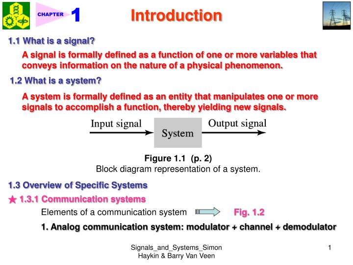
1. CHAPTER. Introduction. 1.1 What is a signal?. A signal is formally defined as a function of one or more variables that conveys information on the nature of a physical phenomenon. 1.2 What is a system?.

E N D
1 CHAPTER Introduction 1.1 What is a signal? A signal is formally defined as a function of one or more variables that conveys information on the nature of a physical phenomenon. 1.2 What is a system? A system is formally defined as an entity that manipulates one or more signals to accomplish a function, thereby yielding new signals. Figure 1.1 (p. 2)Block diagram representation of a system. 1.3 Overview of Specific Systems ★ 1.3.1 Communication systems Fig. 1.2 Elements of a communication system 1. Analog communication system: modulator + channel + demodulator Signals_and_Systems_Simon Haykin & Barry Van Veen
1 CHAPTER Introduction Figure 1.2 (p. 3)Elements of a communication system. The transmitter changes the message signal into a form suitable for transmission over the channel. The receiver processes the channel output (i.e., the received signal) to produce an estimate of the message signal. ◆ Modulation: 2. Digital communication system: sampling + quantization + coding transmitter channel receiver ◆ Two basic modes of communication: Fig. 1.3 • Broadcasting • Point-to-point communication Radio, television Telephone, deep-space communication Signals_and_Systems_Simon Haykin & Barry Van Veen
1 CHAPTER Introduction Figure 1.3 (p. 5)(a) Snapshot of Pathfinder exploring the surface of Mars. (b) The 70-meter (230-foot) diameter antenna located at Canberra, Australia. The surface of the 70-meter reflector must remain accurate within a fraction of the signal’s wavelength. (Courtesy of Jet Propulsion Laboratory.) Signals_and_Systems_Simon Haykin & Barry Van Veen
1 CHAPTER Introduction ★ 1.3.2 Control systems Figure 1.4 (p. 7)Block diagram of a feedback control system. The controller drives the plant, whose disturbed output drives the sensor(s). The resulting feedback signal is subtracted from the reference input to produce an error signal e(t), which, in turn, drives the controller. The feedback loop is thereby closed. ◆ Reasons for using control system: 1. Response, 2. Robustness ◆ Closed-loop control system: Fig. 1.4. Controller: digital computer (Fig. 1.5.) • Single-input, single-output (SISO) system • Multiple-input, multiple-output (MIMO) system Signals_and_Systems_Simon Haykin & Barry Van Veen
1 CHAPTER Introduction Figure 1.5 (p. 8)NASA space shuttle launch.(Courtesy of NASA.) Signals_and_Systems_Simon Haykin & Barry Van Veen
1 CHAPTER Introduction ★ 1.3.3 Microelectromechanical Systems (MEMS) Structure of lateral capacitive accelerometers: Fig. 1-6 (a). Figure 1.6a (p. 8)Structure of lateral capacitive accelerometers.(Taken from Yazdi et al., Proc. IEEE, 1998) Signals_and_Systems_Simon Haykin & Barry Van Veen
1 CHAPTER Introduction SEM view of Analog Device’s ADXLO5 surface-micromachined polysilicon accelerometer: Fig. 1-6 (b). Figure 1.6b (p. 9)SEM view of Analog Device’s ADXLO5 surface-micromachined polysilicon accelerometer. (Taken from Yazdi et al., Proc. IEEE, 1998) Signals_and_Systems_Simon Haykin & Barry Van Veen
1 CHAPTER Introduction ★ 1.3.4 Remote Sensing Remote sensing is defined as the process of acquiring information about an object of interest without being in physical contact with it 1. Acquisition of information = detecting and measuring the changes that the object imposes on the field surrounding it. 2. Types of remote sensor: Radar sensor Infrared sensor Visible and near-infrared sensor X-ray sensor ※ Synthetic-aperture radar (SAR) See Fig. 1.7 Satisfactory operation High resolution Ex. A stereo pair of SAR acquired from earth orbit with Shuttle Imaging Radar (SIR-B) Signals_and_Systems_Simon Haykin & Barry Van Veen
1 CHAPTER Introduction Figure 1.7 (p. 11)Perspectival view of Mount Shasta (California), derived from a pair of stereo radar images acquired from orbit with the shuttle Imaging Radar (SIR-B). (Courtesy of Jet Propulsion Laboratory.) Signals_and_Systems_Simon Haykin & Barry Van Veen
1 CHAPTER Introduction ★ 1.3.5 Biomedical Signal Processing Morphological types of nerve cells:Fig. 1-8. Figure 1.8 (p. 12)Morphological types of nerve cells (neurons) identifiable in monkey cerebral cortex, based on studies of primary somatic sensory and motor cortices. (Reproduced from E. R. Kande, J. H. Schwartz, and T. M. Jessel, Principles of Neural Science, 3d ed., 1991; courtesy of Appleton and Lange.) Signals_and_Systems_Simon Haykin & Barry Van Veen
1 CHAPTER Introduction ◆ Important examples of biological signal: Figure 1.9 (p. 13)The traces shown in (a), (b), and (c) are three examples of EEG signals recorded from the hippocampus of a rat. Neurobiological studies suggest that the hippocampus plays a key role in certain aspects of learning and memory. • Electrocardiogram (ECG) • Electroencephalogram (EEG) Fig. 1-9 Signals_and_Systems_Simon Haykin & Barry Van Veen
1 CHAPTER Introduction ★ Measurement artifacts: 1. Instrumental artifacts 2. Biological artifacts 3. Analysis artifacts ★ 1.3.6 Auditory System Figure 1.10 (p. 14)(a) In this diagram, the basilar membrane in the cochlea is depicted as if it were uncoiled and stretched out flat; the “base” and “apex” refer to the cochlea, but the remarks “stiff region” and “flexible region” refer to the basilar membrane. (b) This diagram illustrates the traveling waves along the basilar membrane, showing their envelopes induced by incoming sound at three different frequencies. Signals_and_Systems_Simon Haykin & Barry Van Veen
1 CHAPTER Introduction ★ The ear has three main parts: • Outer ear: collection of sound • Middle ear: acoustic impedance match between the air and cochlear fluid Conveying the variations of the tympanic membrane (eardrum) 3. Inner ear: mechanical variations → electrochemical or neural signal ★ Basilar membrane: Traveling wave Fig. 1-10. ★ 1.3.7 Analog Versus Digital Signal Processing • Digital approach has two advantages over analog approach: • Flexibility • Repeatability 1.4 Classification of Signals Parentheses (‧) 1. Continuous-time and discrete-time signals Continuous-time signals: x(t) Fig. 1-11. where t = nTs Discrete-time signals: (1.1) Fig. 1-12. Brackets [‧] Signals_and_Systems_Simon Haykin & Barry Van Veen
1 CHAPTER Introduction Figure 1.11 (p. 17)Continuous-time signal. Figure 1.12 (p. 17)(a) Continuous-time signal x(t). (b) Representation of x(t) as a discrete-time signal x[n]. Signals_and_Systems_Simon Haykin & Barry Van Veen
1 CHAPTER Introduction Symmetric about vertical axis 2. Even and odd signals Even signals: (1.2) Odd signals: (1.3) Example 1.1 Antisymmetric about origin Consider the signal Is the signal x(t) an even or an odd function of time? <Sol.> odd function Signals_and_Systems_Simon Haykin & Barry Van Veen
1 CHAPTER Introduction ◆ Even-odd decomposition of x(t): Example 1.2 Find the even and odd components of the signal where <Sol.> Even component: (1.4) (1.5) Odd component: Signals_and_Systems_Simon Haykin & Barry Van Veen
1 CHAPTER Introduction ◆ Conjugate symmetric: A complex-valued signal x(t) is said to be conjugate symmetric if (1.6) Refer to Fig. 1-13 Problem 1-2 Let 3. Periodic and nonperiodic signals (Continuous-Time Case) (1.7) Periodic signals: Figure 1.13 (p. 20)(a) One example of continuous-time signal. (b) Another example of a continuous-time signal. and Fundamental frequency: (1.8) Angular frequency: (1.9) Signals_and_Systems_Simon Haykin & Barry Van Veen
1 CHAPTER Introduction ◆ Example of periodic and nonperiodic signals:Fig. 1-14. Figure 1.14 (p. 21)(a) Square wave with amplitude A = 1 and period T = 0.2s. (b) Rectangular pulse of amplitude A and duration T1. ◆ Periodic and nonperiodic signals (Discrete-Time Case) (1.10) N = positive integer Fundamental frequency of x[n]: (1.11) Signals_and_Systems_Simon Haykin & Barry Van Veen
1 CHAPTER Introduction Figure 1.15 (p. 21)Triangular wave alternative between –1 and +1 for Problem 1.3. ◆ Example of periodic and nonperiodic signals: Fig. 1-16 and Fig. 1-17. Figure 1.16 (p. 22)Discrete-time square wave alternative between –1 and +1. Signals_and_Systems_Simon Haykin & Barry Van Veen
1 CHAPTER Introduction Figure 1.17 (p. 22)Aperiodic discrete-time signal consisting of three nonzero samples. 4. Deterministic signals and random signals A deterministic signal is a signal about which there is no uncertainty with respect to its value at any time. Figure 1.13 ~ Figure 1.17 A random signal is a signal about which there is uncertainty before it occurs. Figure 1.9 5. Energy signals and power signals Instantaneous power: If R = 1 and x(t) represents a current or a voltage, then the instantaneous power is (1.12) (1.14) (1.13) Signals_and_Systems_Simon Haykin & Barry Van Veen
1 CHAPTER Introduction The total energy of the continuous-time signal x(t) is ◆ Discrete-time case: Total energy of x[n]: (1.15) (1.18) Time-averaged, or average, power is Average power of x[n]: (1.16) (1.19) For periodic signal, the time-averaged power is (1.17) (1.20) ★ Energy signal: If and only if the total energy of the signal satisfies the condition ★ Power signal: If and only if the average power of the signal satisfies the condition Signals_and_Systems_Simon Haykin & Barry Van Veen
1 CHAPTER Introduction 1.5 Basic Operations on Signals ★ 1.5.1 Operations Performed on dependent Variables c = scaling factor Amplitude scaling: x(t) (1.21) Discrete-time case: x[n] Performed by amplifier Addition: (1.22) Discrete-time case: Multiplication: Ex. AM modulation (1.23) Differentiation: Figure 1.18 (p. 26)Inductor with current i(t), inducing voltage v(t) across its terminals. Inductor: (1.25) (1.24) Integration: (1.26) Signals_and_Systems_Simon Haykin & Barry Van Veen
1 CHAPTER Introduction Capacitor: (1.27) Figure 1.19 (p. 27)Capacitor with voltage v(t) across its terminals, inducing current i(t). ★ 1.5.2 Operations Performed on independent Variables Time scaling: a >1 compressed 0 < a < 1 expanded Fig. 1-20. Figure 1.20 (p. 27) Time-scaling operation; (a) continuous-time signal x(t), (b) version of x(t) compressed by a factor of 2, and (c) version of x(t) expanded by a factor of 2. Signals_and_Systems_Simon Haykin & Barry Van Veen
1 CHAPTER Introduction Discrete-time case: k = integer Some values lost! Figure 1.21 (p. 28)Effect of time scaling on a discrete-time signal: (a) discrete-time signal x[n] and (b) version of x[n] compressed by a factor of 2, with some values of the original x[n] lost as a result of the compression. Reflection: The signal y(t) represents a reflected version of x(t) about t = 0. Ex. 1-3 Consider the triangular pulse x(t) shown in Fig. 1-22(a). Find the reflected version of x(t) about the amplitude axis (i.e., the origin). <Sol.> Fig.1-22(b). Signals_and_Systems_Simon Haykin & Barry Van Veen
1 CHAPTER Introduction Figure 1.22 (p. 28)Operation of reflection: (a) continuous-time signal x(t) and (b) reflected version of x(t) about the origin. t0 > 0 shift toward right t0 < 0 shift toward left Time shifting: Ex. 1-4 Time Shifting: Fig. 1-23. Figure 1.23 (p. 29)Time-shifting operation: (a) continuous-time signal in the form of a rectangular pulse of amplitude 1.0 and duration 1.0, symmetric about the origin; and (b) time-shifted version of x(t) by 2 time shifts. Signals_and_Systems_Simon Haykin & Barry Van Veen
1 CHAPTER Introduction Discrete-time case: where m is a positive or negative integer ★ 1.5.3 Precedence Rule for Time Shifting and Time Scaling 1. Combination of time shifting and time scaling: (1.28) (1.29) (1.30) 2. Operation order: To achieve Eq. (1.28), 1st step: time shifting 2nd step: time scaling Ex. 1-5 Precedence Rule for Continuous-Time Signal Consider the rectangular pulse x(t) depicted in Fig. 1-24(a). Find y(t)=x(2t + 3). <Sol.> Case 1: Fig. 1-24. Shifting first, then scaling Case 2: Fig. 1-25. Scaling first, then shifting Signals_and_Systems_Simon Haykin & Barry Van Veen
1 CHAPTER Introduction Figure 1.24 (p. 31)The proper order in which the operations of time scaling and time shifting should be applied in the case of the continuous-time signal of Example 1.5. (a) Rectangular pulse x(t) of amplitude 1.0 and duration 2.0, symmetric about the origin. (b) Intermediate pulse v(t), representing a time-shifted version of x(t). (c) Desired signal y(t), resulting from the compression of v(t) by a factor of 2. Signals_and_Systems_Simon Haykin & Barry Van Veen
1 CHAPTER Introduction Figure 1.25 (p. 31)The incorrect way of applying the precedence rule. (a) Signal x(t). (b) Time-scaled signal v(t) = x(2t). (c) Signal y(t) obtained by shifting v(t) = x(2t) by 3 time units, which yields y(t) = x(2(t + 3)). Ex. 1-6 Precedence Rule for Discrete-Time Signal A discrete-time signal is defined by Find y[n] = x[2x + 3]. Signals_and_Systems_Simon Haykin & Barry Van Veen
1 CHAPTER Introduction <Sol.> See Fig. 1-27. Figure 1.27 (p. 33)The proper order of applying the operations of time scaling and time shifting for the case of a discrete-time signal. (a) Discrete-time signal x[n], antisymmetric about the origin. (b) Intermediate signal v(n) obtained by shifting x[n] to the left by 3 samples. (c) Discrete-time signal y[n] resulting from the compression of v[n] by a factor of 2, as a result of which two samples of the original x[n], located at n = –2, +2, are lost. Signals_and_Systems_Simon Haykin & Barry Van Veen
1 CHAPTER Introduction B and a are real parameters 1.6 Elementary Signals ★ 1.6.1 Exponential Signals (1.31) • Decaying exponential, for which a < 0 • Growing exponential, for which a > 0 Figure 1.28 (p. 34)(a) Decaying exponential form of continuous-time signal. (b) Growing exponential form of continuous-time signal. Signals_and_Systems_Simon Haykin & Barry Van Veen
1 CHAPTER Introduction Ex. Lossy capacitor: Fig. 1-29. KVL Eq.: (1.32) RC = Time constant (1.33) Figure 1.29 (p. 35)Lossy capacitor, with the loss represented by shunt resistance R. Discrete-time case: (1.34) where Fig. 1.30 ★ 1.6.2 Sinusoidal Signals Fig. 1-31 ◆Continuous-time case: (1.35) where periodicity Signals_and_Systems_Simon Haykin & Barry Van Veen
1 CHAPTER Introduction Figure 1.30 (p. 35)(a) Decaying exponential form of discrete-time signal. (b) Growing exponential form of discrete-time signal. Signals_and_Systems_Simon Haykin & Barry Van Veen
1 CHAPTER Introduction Figure 1.31 (p. 36)(a) Sinusoidal signal A cos( t + Φ) with phase Φ = +/6 radians. (b) Sinusoidal signal A sin (t + Φ) with phase Φ = +/6 radians. Signals_and_Systems_Simon Haykin & Barry Van Veen
1 CHAPTER Introduction Ex. Generation of a sinusoidal signal Fig. 1-32. Circuit Eq.: (1.36) (1.37) where Figure 1.32 (p. 37)Parallel LC circuit, assuming that the inductor L and capacitor C are both ideal. (1.38) Natural angular frequency of oscillation of the circuit ◆Discrete-time case : (1.39) Periodic condition: (1.40) or (1.41) Ex. A discrete-time sinusoidal signal: A = 1, = 0, and N = 12. Fig. 1-33. Signals_and_Systems_Simon Haykin & Barry Van Veen
1 CHAPTER Introduction Figure 1.33 (p. 38)Discrete-time sinusoidal signal. Signals_and_Systems_Simon Haykin & Barry Van Veen
1 CHAPTER Introduction Example 1.7 Discrete-Time Sinusoidal Signal A pair of sinusoidal signals with a common angular frequency is defined by and • Both x1[n] and x2[n] are periodic. Find their common fundamental period. • Express the composite sinusoidal signal In the form y[n] = Acos(n + ), and evaluate the amplitude A and phase . <Sol.> (a) Angular frequency of both x1[n] and x2[n]: This can be only for m = 5, 10, 15, …, which results in N = 2, 4, 6, … (b) Trigonometric identity: Let = 5, then compare x1[n] + x2[n] with the above equation to obtain that Signals_and_Systems_Simon Haykin & Barry Van Veen
1 CHAPTER Introduction • = / 6 Accordingly, we may express y[n] as ★ 1.6.3 Relation Between Sinusoidal and Complex Exponential Signals 1. Euler’s identity: (1.41) (1.42) Complex exponential signal: (1.35) (1.42) Signals_and_Systems_Simon Haykin & Barry Van Veen
1 CHAPTER Introduction ◇ Continuous-time signal in terms of sine function: (1.44) (1.45) 2. Discrete-time case: (1.46) and (1.47) 3. Two-dimensional representation of the complex exponential e j n for = /4 and n = 0, 1, 2, …, 7. : Fig. 1.34. Projection on real axis: cos(n); Projection on imaginary axis: sin(n) Figure 1.34 (p. 41)Complex plane, showing eight points uniformly distributed on the unit circle. Signals_and_Systems_Simon Haykin & Barry Van Veen
1 CHAPTER Introduction ★ 1.6.4 Exponential Damped Sinusoidal Signals (1.48) Example for A = 60, = 6, and = 0: Fig.1.35. Figure 1.35 (p. 41)Exponentially damped sinusoidal signal Ae at sin(t), with A = 60 and = 6. Signals_and_Systems_Simon Haykin & Barry Van Veen
1 CHAPTER x[n] 1 n 3 2 1 0 1 2 3 4 Introduction Ex. Generation of an exponential damped sinusoidal signal Fig. 1-36. Circuit Eq.: (1.49) (1.50) where (1.51) Figure 1.36 (p. 42)Parallel LRC, circuit, with inductor L, capacitor C, and resistor R all assumed to be ideal. Comparing Eq. (1.50) and (1.48), we have ◆ Discrete-time case: (1.52) ★ 1.6.5 Step Function Figure 1.37 (p. 43)Discrete-time version of step function of unit amplitude. ◆ Discrete-time case: (1.53) Fig. 1-37. Signals_and_Systems_Simon Haykin & Barry Van Veen
1 CHAPTER Introduction ◆ Continuous-time case: Figure 1.38 (p. 44)Continuous-time version of the unit-step function of unit amplitude. (1.54) Example 1.8 Rectangular Pulse Consider the rectangular pulse x(t) shown in Fig. 1.39 (a). This pulse has an amplitude A and duration of 1 second. Express x(t) as a weighted sum of two step functions. <Sol.> 1. Rectangular pulse x(t): (1.55) (1.56) Example 1.9 RC Circuit Find the response v(t) of RC circuit shown in Fig. 1.40 (a). <Sol.> Signals_and_Systems_Simon Haykin & Barry Van Veen
1 CHAPTER Introduction Figure 1.39 (p. 44)(a) Rectangular pulse x(t) of amplitude A and duration of 1 s, symmetric about the origin. (b) Representation of x(t) as the difference of two step functions of amplitude A, with one step function shifted to the left by ½ and the other shifted to the right by ½; the two shifted signals are denoted by x1(t) and x2(t), respectively. Note that x(t) = x1(t) – x2(t). Signals_and_Systems_Simon Haykin & Barry Van Veen
1 CHAPTER Introduction Figure 1.40 (p. 45)(a) Series RC circuit with a switch that is closed at time t = 0, thereby energizing the voltage source. (b) Equivalent circuit, using a step function to replace the action of the switch. 1. Initial value: 2. Final value: 3. Complete solution: (1.57) Signals_and_Systems_Simon Haykin & Barry Van Veen
1 CHAPTER (t) a(t) Figure 1.41 (p. 46)Discrete-time form of impulse. Introduction Figure 1.41 (p. 46)Discrete-time form of impulse. ★ 1.6.6 Impulse Function ◆ Discrete-time case: (1.58) Fig. 1.41 Figure 1.42 (p. 46)(a) Evolution of a rectangular pulse of unit area into an impulse of unit strength (i.e., unit impulse). (b) Graphical symbol for unit impulse. (c) Representation of an impulse of strength a that results from allowing the duration Δ of a rectangular pulse of area a to approach zero. Signals_and_Systems_Simon Haykin & Barry Van Veen
1 CHAPTER Introduction ◆ Continuous-time case: Dirac delta function (1.59) (1.60) 1. As the duration decreases, the rectangular pulse approximates the impulse more closely. Fig. 1.42. 2. Mathematical relation between impulse and rectangular pulse function: • x(t): even function of t, = duration. • x(t): Unit area. (1.61) Fig. 1.42 (a). 3. (t) is the derivative of u(t): 4. u(t) is the integral of (t): (1.62) (1.63) Example 1.10 RC Circuit (Continued) For the RC circuit shown in Fig. 1.43 (a), determine the current i (t) that flows through the capacitor for t 0. Signals_and_Systems_Simon Haykin & Barry Van Veen
1 CHAPTER Introduction <Sol.> Figure 1.43 (p. 47)(a) Series circuit consisting of a capacitor, a dc voltage source, and a switch; the switch is closed at time t = 0. (b) Equivalent circuit, replacing the action of the switch with a step function u(t). 1. Voltage across the capacitor: 2. Current flowing through capacitor: Signals_and_Systems_Simon Haykin & Barry Van Veen
1 CHAPTER Introduction ◆ Properties of impulse function: (1.68) 1. Even function: (1.64) 2. Sifting property: Ex. RLC circuit driven by impulsive source: Fig. 1.45. (1.65) 3. Time-scaling property: For Fig. 1.45 (a), the voltage across the capacitor at time t = 0+ is (1.66) (1.69) <p.f.> Fig. 1.44 1. Rectangular pulse approximation: (1.67) 2. Unit area pulse: Fig. 1.44(a). Time scaling: Fig. 1.44(b). Area = 1/a Restoring unit area ax(at) Signals_and_Systems_Simon Haykin & Barry Van Veen
1 CHAPTER Introduction Figure 1.44 (p. 48)Steps involved in proving the time-scaling property of the unit impulse. (a) Rectangular pulse xΔ(t) of amplitude 1/Δ and duration Δ, symmetric about the origin. (b) Pulse xΔ(t) compressed by factor a. (c) Amplitude scaling of the compressed pulse, restoring it to unit area. Figure 1.45 (p. 49)(a) Parallel LRC circuit driven by an impulsive current signal. (b) Series LRC circuit driven by an impulsive voltage signal. Signals_and_Systems_Simon Haykin & Barry Van Veen
1 CHAPTER Introduction ★ 1.6.7 Derivatives of The Impulse Problem 1.24 1. Doublet: (1.70) 2. Fundamental property of the doublet: (1.71) (1.72) 3. Second derivative of impulse: (1.73) ★ 1.6.8 Ramp Function 1. Continuous-time case: (1.74) Fig. 1.46 or (1.75) Signals_and_Systems_Simon Haykin & Barry Van Veen
1 CHAPTER x[n] 4 n 3 2 1 0 1 2 3 4 Introduction 2. Discrete-time case: Figure 1.46 (p. 51)Ramp function of unit slope. (1.76) or (1.77) Fig. 1.47. Figure 1.47 (p. 52)Discrete-time version of the ramp function. Example 1.11 Parallel Circuit Consider the parallel circuit of Fig. 1-48 (a) involving a dc current source I0 and an initially uncharged capacitor C. The switch across the capacitor is suddenly opened at time t = 0. Determine the current i(t) flowing through the capacitor and the voltage v(t) across it for t 0. <Sol.> 1. Capacitor current: Signals_and_Systems_Simon Haykin & Barry Van Veen