Download
1 / 33
330 likes | 455 Vues
Long-range Dependency Effects in Network Timekeeping. David L. Mills University of Delaware http://www.eecis.udel.edu/~mills mailto:mills@udel.edu. Sources of error in network timekeeping. Short-range distribution induced errors

E N D
Long-range Dependency Effects in Network Timekeeping David L. Mills University of Delaware http://www.eecis.udel.edu/~mills mailto:mills@udel.edu
Sources of error in network timekeeping • Short-range distribution induced errors • Software latencies due to cache misses, context switches, page faults and process scheduling • Hardware latencies due to interrupts, network collisions, nonmaskable interrupts and timer/clock resolution • Asymmetric network propagation paths to and from the server • Suspected long-range distribution induced errors • Network propagation path delay and jitter. • Jitter induced by wander in the system clock oscillator • We need to prove/disprove whether long-range effects are in play.
Jitter witn a serial port hardware and driver • Graph shows raw jitter of millisecond timecode and 9600-bps serial port. Samples are uniformly distributed over the character interval. • Additional latencies from 1.5 ms to 8.3 ms on SPARC IPC due to software driver and operating system; rare latency peaks over 20 ms • Using on-second format and median filter, residual jitter is less than 50 ms
Jitter with a PPS signal and Digital Alpha 433 • Graph shows raw jitter of PPS timecode and parallel port due to interrupt latencies. • While not proven, the distribution looks very much like exponential. • Standard deviation 51.3 ns
Jitter with a modem and ACTS service • Measurements use 2400-bps telephone modem and NIST Automated Computer Time Service (ACTS). Calls are placed at 16,384-s intervals. • Jitter is due primarily due to digital processing in the modem. • It is not clear what the distribution is, but it could include LRD.
Computing and filtering offset and delay samples T2 Server T3 • The most accurate offset q0 is measured at the lowest delay d0 (apex of the wedge scattergram). • The correct time q must lie within the wedge q0 ± (d - d0)/2. • The d0 is estimated as the minimum of the last eight delay measurements and (q0 ,d0) becomes the peer update. • Each peer update can be used only once and must be more recent than the previous update. x q0 T1 Client T4
Clock filter performance • Left figure shows raw time offsets measured for a typical path over a 24-hour period (mean error 724 ms, median error 192 ms) • Right graph shows filtered time offsets over the same period (mean error 192 ms, median error 112 ms). • The mean error has been reduced by 11.5 dB; the median error by 18.3 dB. This is impressive performance.
Asymmetric path delays • We like to think that the delays on the outbound and inbound network paths are the same, or at least drawn from the same distribution. • Such is not the case in several instances, one of which is shown in the wedge scattergram on the next slide. • The occasion arises with a slow PPP line while downloading a large file. • The download direction utilization is essentially 100 percent, while the other direction carries only ACKs and is only minimally utilized. • The delay distribution on the download direction depends on the packet length distribution, which is SRD. • The delay distribution on the other direction depends on the network jitter, which may or may not be LRD.
Raw roundtrip delay distribution function from survey • Cumulative distribution function of absolute roundtrip delays • 38,722 Internet servers surveyed running NTP Version 2 and 3 • Delays: median 118 ms, mean 186 ms, maximum 1.9 s(!) • Asymmetric delays can cause errors up to one-half the delay
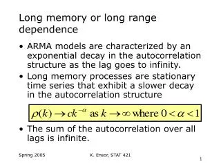
Self-similar distributions • Consider the (continuous) process X = (Xt, -∞ < t < ∞) • If Xat and aH(Xt) have identical finite distributions for a > 0, then X is self-similar with parameter H. • We need to apply this concept to a time series. Let X = (Xt, t = 0, 1, …) with given mean m, variance s2 and autocorrelation function r(k), k≥ 0. • It’s convienent to express this as r(k) = k-bL(k) as k→∞ and 0 < b < 1. • We assume L(k) varies slowly near infinity and can be assumed a constant like 1.
Definition of self-similar distribution • For m = 1, 2, … let X (m) = (Xk (m) , k = 1, 2, …), where m is a scale factor. • Each Xk (m) represents a subinterval of m samples, and the subintervals are non-overlapping: Xk (m) = 1 / m (X (m)(k – 1) m , + … + X (m)km – 1), k > 0. • For instance, m = 2 subintervals are (0,1), (2,3), …; m = 3 subintervals are (0, 1, 2), (3, 4, 5), … • A process is (exactly) self-similar with parameter H = 1 – b / 2 if, for all m = 1, 2, …, var[X(m)] = s2m – b and r(m)(k) = r(k) = 1 / 2 [(k + 1)2H – 2k2H + (k – 1)2H], k > 0, where r(m) represents the autocorrelation function of X (m). • A process is (asymptotically) second-order self-similar if r(m)(k) -> r(k) as m→∞. • Plot r(k) = k-b = k1 – 2H in log-log coordinates as a straight line with • b = -1 for H = 0.5, representing short-range dependent (SRD) distribution, • -1 < b < 0 for 0.5 < H < 1, representing long-range dependent (LRD) distribution, • b = 1 for H = 1, representing a random-walk distribution.
Properties of self-similar distributions • For self-similar distributions (0.5 < H < 1) • Hurst effect: the rescaled, adjusted range statistic is characterized by a power law; i.e., E[R(m) / S(m)] is similar to mH as m→∞. • Slowly decaying variance. the variances of the sample means are decaying more slowly than the reciprocal of the sample size. • Long-range dependence: the autocorrelations decay hyperbolically rather than exponentially, implying a non-summable autocorrelation function. • 1 / f noise: the spectral density f(.) obeys a power law near the origin. • For memoryless or finite-memory distributions (0 < H < 0.5 ) • var[X (m)] decays as to m-1. • The sum of variances if finite. • The spectral density f(.) is finite near the origin.
Origins of self-similar processes • Long-range dependent (0.5 < H < 1) • Fractional Gaussian Noise (F-GN) r(k) = 1 / 2 [(k + 1)2H – 2k2H+ (k – 1)2H], k > 1 • Fractional Brownian Motion (F-BM) • Fractional Autoregressive Integrative Moving Average (F-ARIMA • Random Walk (RW) (descrete Brownian Motion (BM)) • Short-range dependent • Memoryless and short-memory (Markov) • Just about any conventional distribution – uniform, exponential, Pareto • ARIMA
Simulation studies • The object of these simulations is to confirm samples from a given distribution have short-range dependency (SRD) or long-range dependency (LRD). • X is a time series of N samples drawn from a distribution with given mean m and variance s. • X (m) = (Xk (m), k = 1, 2, …), where m = 1, 2, 4, … is a scale factor increasing in powers of two. • X is divided in contiguous, non-overlapping intervals of size m indexed by k. • a(m) = (ak (m), k = 1, 2, …) is the time series corresponding to the average of the samples in each interval . • The variance-time graph plots variance s2(a(m)) against m in log-log scales. m = 1 X1 X2 X3 X4 X5 X6 X7 X8 … k m = 2 k (X1 + X2) / 2 (X3 + X4) / 2 (X5 + X6) / 2 (X7 + X8) / 2 …
Exponential distribution • The object of this experiment is to determine whether an exponential distribution has only SRD. • 100,000 samples generated from an exponential distribution with s = 1. • The next slide shows the time series Xk (m) for values of m = 1, 4, 16 and 64. Note the weak self-similar characteristic. • The second slide shows the variance-time plot, which shows the Hurst parameter H = 0.5 and confirms the exponential distribution has only SRD. • This property is true also of other processes generated by uniform, Poisson, finite Markov and just about every other process without a heavy-tail autocorrelation function.
Exponential distribution variance-time plot • Graph shows the variance from data averaged over specified intervals. • One curve shows the data, the other shows SRD with H = 0.5. • Both curves overlap almost everywhere, showing the distribution is SRD.
Random-walk distribution • The object of this experiment is to determine whether a random-walk distribution is LRD. • 1,000,000 samples were generated from a random-walk distribution consisting of the integral of a Gaussian distribution with m = 0 and s = 0.1. • The next slide shows the time series Xk (m) for m = 1, 16, 256 and 4096 seconds. Note the curves of the first three are almost identical, except for some high-frequency smoothing at m = 4096. • This is to be expected, since even at m = 4096 the intervals are small compared to the wiggle of the curve. This is characteristic of flicker (1 / f) noise and the fact the autocorrelation functions are non-summable. • Random-walk distributions (H = 1) are probably not good models for network delays, but they are good models for computer clock oscillator wander.
Filtered exponential distribution • A strict random-walk distribution ( H = 1) is probably not a good model for network delays. A better model would have H somewhere in the middle of 0.5 < H < 1. • Generating a strict self-similar time series for given H is computationally complex and expensive. • So, try a filtered exponential distribution with given finite autocorrelation function r(k) = kb (1 ≤k≤n, 0 ≤b≤ 1). We choose n = 1,000 and b = 1. • The next slide shows the time series Xk (m) for m = 1, 16, 256 and 1024 seconds. Note the curves of the first three are almost identical. There is some decay at 1024 s. • The variance-time plot on the second page shows random-walk and characteristic at lags in the order of n and decays to SRD after tha.
Filtered exponential distribution variance-time plot • Graph shows the variance from data averaged over specified intervals. • The upper curve from data shows filtered exponential. • The lower curve shows SRD with H = 0.5 for reference.
Experiment study – USNO data • The object of this experiment is to determine whether roundtrip delays measured over Internet paths by NTP show long-range dependency. • The Internet path was between primary time servers pogo.udel.edu at UDel and tick.usno.navy.mil in Washington, DC. • Measurements were made every 16 seconds over about 11 days. • The next slide shows the path delays are asymmetric. The roundtrip delay is the sum of the two one-way delays, which is the convolution of their distributions. In most cases we assume the two distributionsare the same. • The following slide shows the smoothed delay at averaging intervals m = 32, 64, 64 and 256 seconds. Note the weak self-similar characteristic.
USNO data wedge scattergram • Each dot represents a offset/delay sample. • The upper limb of the wedge represents packets inbound to USNO; the lower limb outbount. • Obviously, the traffic is asymmetric, so the delays should be as well.
USNO data delay variance-time plot • Graph shows the variance from data averaged over specified intervals. • The upper curve from data shows LRD with 0.5 < H < 1. • The lower curve shows SRD with H = 0.5 for reference.
Data from Levine paper • The following figures are from the paper: • Levine, W.E., M.S. Taqqu, W. Willinger and D.V. Wilson. On the self-similar nature of Ethernet traffic (extended version). IEEE/ACM Trans. Networking 2, 1 (February 1984), 1-15. • They show the same thing, that network delay distributions have LRD in some degree or other. • The next slide shows an example of a self-similar distribution at five different values of m for network traffic (left) and samples drawn from an exponential distribution (right). • The fact those on the left look substantially “like each other” suggests the distribution has more LRD than SRD. • The fact those on the right look very different suggests the underlying distribution has more SRD and LRD.
Variance-time plot • This is a variance-time plot from the network traffic. The lower line is for H = 0.5. Apparently, the network traffic has LRD 0.5 < H < 1.
R/S plot • This is a S/R (poc) plot from the network traffic. This further confirms the network traffic has LRD 0.5 < H < 1.
Periodogram (discrete Fourier transform) plot • This is a periodogram (Fourier transform) from the network traffic. this further confirms the network traffic has LRD 0.5 < H < 1.