Download
1 / 36
360 likes | 514 Vues
RNA. CS 466 Saurabh Sinha. RNA. RNA is similar to DNA chemically. It is usually only a single strand. T(hyamine) is replaced by U(racil) Some forms of RNA can form secondary structures by “ pairing up ” with itself. This can change its properties dramatically. tRNA linear and 3D view:.

E N D
RNA CS 466 Saurabh Sinha
RNA • RNA is similar to DNA chemically. It is usually only a single strand. T(hyamine) is replaced by U(racil) • Some forms of RNA can form secondary structures by “pairing up” with itself. This can change its properties dramatically. tRNA linear and 3D view: http://www.cgl.ucsf.edu/home/glasfeld/tutorial/trna/trna.gif
RNA • There’s more to RNA than mRNA • RNA can adopt interesting non-linear structures, and catalyze reactions • tRNAs (transfer RNAs) are the “adapters” that implement translation • More recently, found to have various regulatory effects on gene expression
Secondary structure • Several interesting RNAs have a conserved secondary structure (resulting from base-pairing interactions) • Sometimes, the sequence itself may not be conserved for the function to be retained • It is important to tell what the secondary structure is going to be, for homology detection
Conserved secondary structure N-Y A A N-N’ N-N’ R N-N’ N-N’ N-N’ N-N’ N-N’ / N Consensus binding site for R17 phage coat protein. N = A/C/G/U, N’ is a complementary base pairing to N, Y is C/U, R is A/G Source: DEKM
Basics of secondary structure • G-C pairing: three bonds (strong) • A-U pairing: two bonds (weaker) • Base pairs are approximately coplanar
Basics of secondary structure • G-C pairing: three bonds (strong) • A-U pairing: two bonds (weaker) • Base pairs are approximately coplanar • Base pairs are stacked onto other base pairs (arranged side by side): “stems”
Secondary structure elements loop at the end of a stem stem loop … on both sides of stem single stranded bases within a stem … only on one side of stem Loop: single stranded subsequences bounded by base pairs
Non-canonical base pairs • G-C and A-U are the canonical base pairs • G-U is also possible, almost as stable
Nesting • Base pairs almost always occur in a nested fashion • If positions i and j are paired, and positions i’ and j’ are paired, then these two base-pairings are said to be nested if: • i < i’ < j’ < j OR i’ < i < j < j’ • Non-nested base pairing: pseudoknot
Pseudoknot (9, 18) (2, 11) NOT NESTED 9 18 11 2
Pseudoknot problems • Pseudoknots are not handled by the algorithms we shall see • Pseudoknots do occur in many important RNAs • But the total number of pseudoknotted base pairs is typically relatively small
Secondary structure predictionApproach 1. • Find the secondary structure with most base pairs. • Nussinov’s algorithm • Recursive: finds best structure for small subsequences, and works its way outwards to larger subsequences
Nussinov’s algorithm: idea • There are only four possible ways of getting the best structure for subsequence (i,j) from the best structures of the smaller subsequences
Nussinov’s algorithm: idea • There are only four possible ways of getting the best structure for subsequence (i,j) from the best structures of the smaller subsequences (1) Add unpaired position i onto best structure for subsequence (i+1,j) i+1 j i
Nussinov’s algorithm: idea • There are only four possible ways of getting the best structure for subsequence (i,j) from the best structures of the smaller subsequences (2) Add unpaired position j onto best structure for subsequence (i,j-1) i j-1 j
Nussinov’s algorithm: idea • There are only four possible ways of getting the best structure for subsequence (i,j) from the best structures of the smaller subsequences (3) Add (i,j) pair onto best structure for subsequence (i+1,j-1) i+1 j-1 i j
Nussinov’s algorithm: idea • There are only four possible ways of getting the best structure for subsequence (i,j) from the best structures of the smaller subsequences (4)Combine two optimal substructures (i,k) and (k+1,j) i k k+1 j
Nussinov RNA folding algorithm • Given a sequence s of length L with symbols s1 … sL. Let (i,j) = 1 if si and sj are a complementary base pair, and 0 otherwise. • We recursively calculate scores g(i,j) which are the maximal number of base pairs that can be formed for subsequence si…sj. • Dynamic programming
Recursion • Starting with all subsequences of length 2, to length L • g(i,j) = max of • g(i+1, j) • g(i,j-1) • g(i+1,j-1) + (i,j) • maxi < k < j [g(i,k) + g(k+1,j)] • Initialization • g(i,i-1) = 0 • g(i,i) = 0 O(n2) ? No. O(n3)
Traceback • As usual in sequence alignment ? • Optimal sequence alignment is a linear path in the dynamic programming table • Optimal secondary structure can have “bifurcations” • Traceback uses a pushdown stack
Traceback Push (1,L) onto stack Repeat until stack is empty: pop (i,j) if i >= j continue else if g(i+1,j) = g(i,j) push (i+1,j) else if g(i,j-1) = g(i,j) push (i,j-1) else if g(i+1,j-1) + (i,j) = g(i,j) record (i,j) base pair push (i+1,j-1) else for k = i+1 to j-1, if g(i,k)+g(k+1,j) g(i,j) push (k+1,j) push (i,k) break (for loop)
Secondary structure predictionApproach 2 • Based on minimization of ∆G, the equilibrium free energy, rather than maximization of number of base pairs • Better fit to real (experimental) ∆G • Energy of stem is sum of “stacking” contributions from the interface between neighboring base pairs
Source: DEKM U U A A G-C G-C A G-C U-A A-U C-G A-U A A 4nt loop +5.9 -1.1 terminal mismatch of hairpin -2.9 stack 1nt bulge +3.3 -2.9 stack (special case) -1.8 stack -0.9 stack -1.8 stack -2.1 stack dangle -0.3 • Neighboring base pairs: stack • Single bulges OK in stacking • Longer bulges: no stacking term • Loop destabilisation energy • Loop terminal mismatch energy
hairpin loop: exactly one base pair internal loop: exactly two base pairs bulge: internal loop with one base from each base pair being adjacent multibranched loop: > 2 base pairs in a loop, one base pair is closest to ends of RNA. this is the “exterior” or “closing” base pair all other base pairs are “interior” Source: Martin Tompa’s lecture notes
Energy contributions • eS(i,j): Free energy of stacked pair (i,j) and (i+1,j-1) • eH(i,j): Free energy of a hairpin loop closed by (i,j): depends on length of loop, bases at i,j, and bases adjacent to them • eL(i,j,i’,j’): Free energy of an internal loop or bulge, with (i,j) and (i’,j’) being the bordering base pairs. Depends on bases at these positions, and unpaired bases adjacent to them • eM(i,j,i1,j1,…ik,jk): Free energy of a multibranch loop with (i,j) as the closing base pair and i1j1 etc as the internal base pairs
Zuker’s algorithm:Dynamic programming • W(j): FE of optimal structure of s[1..j] • V(i,j): FE of optimal structure of s[i..j] assuming i,j form a base pair • VBI(i,j): FE of optimal structure of s[i..j] assuming i,j closes a bulge or internal loop • VM(i,j): FE of optimal structure of s[i..j] assuming i,j closes a multibranch loop • WM(i,j): used to compute VM
s[j] is external base (a base not in any loop) s[j] pairs with s[i], for some i < j Dynamic programming recurrences • W(j): FE of optimal structure of s[1..j] • W(0) = 0 • W(j) = min( W(j-1), min1<=i<jV(i,j)+W(i-1))
Dynamic programming recurrences • V(i,j): FE of optimal structure of s[i..j] assuming i,j form a base pair • V(i,j) = infinity if i >= j • V(i,j) = min( eH(i,j), eS(i,j) + V(i+1,j-1), VBI(i,j), VM(i,j)) if i < j i,j is exterior base pair of a hairpin loop
Dynamic programming recurrences • V(i,j): FE of optimal structure of s[i..j] assuming i,j form a base pair • V(i,j) = infinity if i >= j • V(i,j) = min( eH(i,j), eS(i,j) + V(i+1,j-1), VBI(i,j), VM(i,j)) if i < j i,j is exterior pair of a stacked pair. i+1,j-1 is therefore a pair too.
Dynamic programming recurrences • V(i,j): FE of optimal structure of s[i..j] assuming i,j form a base pair • V(i,j) = infinity if i >= j • V(i,j) = min( eH(i,j), eS(i,j) + V(i+1,j-1), VBI(i,j), VM(i,j)) if i < j i,j is exterior pair of a bulge or interior loop
Dynamic programming recurrences • V(i,j): FE of optimal structure of s[i..j] assuming i,j form a base pair • V(i,j) = infinity if i >= j • V(i,j) = min( eH(i,j), eS(i,j) + V(i+1,j-1), VBI(i,j), VM(i,j)) if i < j i,j is exterior pair of a multibranch loop
Dynamic programming recurrences • VBI(i,j): FE of optimal structure of s[i..j] assuming i,j closes a bulge or internal loop • VBI(i,j) = min (eL(i,j,i’,j’) + V(i’,j’)) • Slow ! i’,j’ i<i’<j’<j Energy of the bulge
Dynamic programming recurrences • VM(i,j): FE of optimal structure of s[i..j] assuming i,j closes a multibranch loop • VM(i,j) = min (eM(i,j,i1,j1,..,ik,jk) + ∑hV(ih,jh)) • Very slow ! k>=2 i1,j1,…ik,jk Energy of the loop itself
Order of computation • What order to fill the DP table in ? • Increasing order of (j-i) • VBI(i,j) and VM(i,j) before V(i,j)