Download
1 / 13
150 likes | 306 Vues
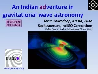
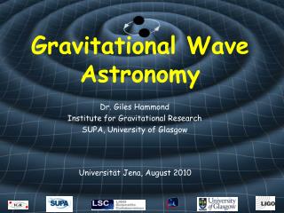
Gravitational Wave Astronomy. Dr. Giles Hammond Institute for Gravitational Research SUPA, University of Glasgow. Universität Jena, August 2010. Statistical techniques are used to analyse analyse data from detectors Consider a measurement of a sine wave in the presence of noise

E N D
Gravitational Wave Astronomy Dr. Giles Hammond Institute for Gravitational Research SUPA, University of Glasgow Universität Jena, August 2010
Statistical techniques are used to analyse analyse data from detectors Consider a measurement of a sine wave in the presence of noise white noise (mean=0, =0.5) + small signal ( ) = very noisy data Data Analysis
How can we recover the signal (if at all?) Assume our 35Hz sine wave is sampled at 35kHz (16kHz in most detectors) => 1 cycle contains 1000 samples Averaging approximately 150 samples (7 points per cycle) gives Data Analysis
Averaging approximately 150 samples (7 points per cycle) gives Can recover a sinusiodal variation with correct frequency Data Analysis
But there are better ways than straightforward averaging 1) Take a FFT (Fast Fourier Transform) This is a good way to utilise a stream of data Fourier transform for continuous data Fourier transform (FFT) for discrete data Data Analysis
But there are better ways than straightforward averaging 1) Take a FFT (Fast Fourier Transform) This is a good way to utilise a stream of data Data Analysis 35 Hz is clearly visible above the noise The component of white noise at a particular frequency is small => godd to use FFT
2) Take a cross-correlation with a known waveform This is similar to what is done in a Lock-In amplifier (the reference is the known waveform used for the search) We need to know the waveform => modelling required Data Analysis
2) Cross-correlation of random noise X = Data Analysis Average value of cross-correlation is zero The envelope is due to zero padding
2) Cross-correlation of noisy signal with known waveform X = Data Analysis Average value of cross-correlation is non-zero Periodicity due to sine wave
In practice data analysists utilises multiple techniques Burst sources => power spectrum approach or look for excess power in the data Continuous sources => FFT, averaging and cross correlation (using Electro-Magnetic observations for phase of pulsar) Binary Mergers => FFT and cross correlation Data Analysis
Data Analysis complicated by the fact that: Detector noise is not always Gaussian or stationary (the mean and spectral content of the noise vary) Signals are modulated by doppler shifts due to orbital dynamics The detector sensitivity pattern is modulated by the Earth’s rotation (F+ and Fx for the polarisations) Data Analysis
Bar Detectors • Consider that the bar detector is made from two masses separated by a spring (the bar material) • Typically M is 1500kg and the resonant frequency is 1kHz • In the presence of a gravitational tidal force (Fg) and non-gravitational forces (Fng) the equation of motion is M/2 M/2
Bar Detectors • We previously saw that the change in proper separation is • and the wave stretches the spring with a tidal force • and the result is a simple harmonic oscillator driven by the gravitational wave tidal force.