Download
1 / 90
900 likes | 1.1k Vues
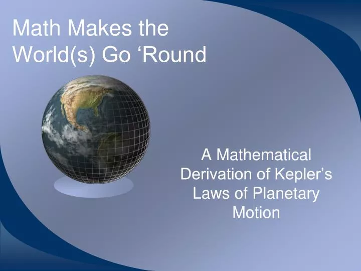
Math Makes the World(s) Go ‘Round. A Mathematical Derivation of Kepler’s Laws of Planetary Motion. by Dr. Mark Faucette. Department of Mathematics University of West Georgia. A Little History. A Little History.

E N D
Math Makes the World(s) Go ‘Round A Mathematical Derivation of Kepler’s Laws of Planetary Motion
by Dr. Mark Faucette Department of Mathematics University of West Georgia
A Little History Modern astronomy is built on the interplay between quantitative observations and testable theories that attempt to account for those observations in a logical and mathematical way.
A Little History In his books On the Heavens, and Physics, Aristotle (384-322 BCE)put forward his notion of an ordered universe or cosmos.
A Little History In the sublunary region, substances were made up of the four elements, earth, water, air, and fire.
A Little History Earth was the heaviest, and its natural place was the center of the cosmos; for that reason the Earth was situated in the center of the cosmos.
A Little History Heavenly bodies were part of spherical shells of aether. These spherical shells fit tightly around each other in the following order: Moon, Mercury, Venus, Sun, Mars, Jupiter, Saturn, fixed stars.
A Little History In his great astronomical work, Almagest, Ptolemy (circa 200) presented a complete system of mathematical constructions that accounted successfully for the observed motion of each heavenly body.
A Little History Ptolemy used three basic construc- tions, the eccentric, the epicycle, and the equant.
A Little History With such combinations of constructions, Ptolemy was able to account for the motions of heavenly bodies within the standards of observational accuracy of his day.
A Little History However, the Earth was still at the center of the cosmos.
A Little History About 1514, Nicolaus Copernicus (1473-1543) distributed a small book, the Little Commentary, in which he stated The apparent annual cycle of movements of the sun is caused by the Earth revolving round it.
A Little History A crucial ingredient in the Copernican revolution was the acquisition of more precise data on the motions of objects on the celestial sphere.
A Little History A Danish nobleman, Tycho Brahe (1546-1601), made im-portant contribu- tions by devising the most precise instruments available before the invention of the telescope for observing the heavens.
A Little History The instruments of Brahe allowed him to determine more precisely than had been possible the detailed motions of the planets. In particular, Brahe compiled extensive data on the planet Mars.
A Little History He made the best measurements that had yet been made in the search for stellar parallax. Upon finding no parallax for the stars, he (correctly) concluded that either • the earth was motionless at the center of the Universe, or • the stars were so far away that their parallax was too small to measure.
A Little History Brahe proposed a model of the Solar System that was intermediate between the Ptolemaic and Copernican models (it had the Earth at the center).
A Little History Thus, Brahe's ideas about his data were not always correct, but the quality of the observations themselves was central to the development of modern astronomy.
A Little History Unlike Brahe, Johannes Kepler (1571-1630) believed firmly in the Copernican system.
A Little History Kepler was forced finally to the realization that the orbits of the planets were not the circles demanded by Aristotle and assumed implicitly by Copernicus, but were instead ellipses.
A Little History Kepler formulated three laws which today bear his name: Kepler’s Laws of Planetary Motion
Kepler’s First Law The orbits of the planets are ellipses, with the Sun at one focus of the ellipse. Kepler’s Laws
Kepler’s Second Law The line joining the planet to the Sun sweeps out equal areas in equal times as the planet travels around the ellipse. Kepler’s Laws
Kepler’s Third Law The ratio of the squares of the revolutionary periods for two planets is equal to the ratio of the cubes of their semimajor axes: Kepler’s Laws
Mathematical Derivation of Kepler’s Law Kepler’s Laws can be derived using the calculus from two fundamental laws of physics: • Newton’s Second Law of Motion • Newton’s Law of Universal Gravitation
Newton’s Second Law of Motion The relationship between an object’s mass m, its acceleration a, and the applied force F is F=ma. Acceleration and force are vectors (as indicated by their symbols being displayed in bold font); in this law the direction of the force vector is the same as the direction of the acceleration vector.
Newton’s Law of Universal Gravitation • For any two bodies of masses m1 and m2, the force of gravity between the two bodies can be given by the equation: • where d is the distance between the two objects and G is the constant of universal gravitation.
Choosing the Right Coordinate System Just as we have two distinguished unit vectors i and j corresponding to the Cartesian coordinate system, we can likewise define two distinguished unit vectors ur and uθ corresponding to the polar coordinate system:
Choosing the Right Coordinate System Taking derivatives, notice that
Choosing the Right Coordinate System Now, suppose θ is a function of t, so θ= θ(t). By the Chain Rule,
Choosing the Right Coordinate System For any point r(t) on a curve, let r(t)=||r(t)||, then
Choosing the Right Coordinate System Now, add in a third vector, k, to give a right-handed set of orthogonal unit vectors in space:
Position, Velocity, and Acceleration Recall Also recall the relationship between position, velocity, and acceleration:
Position, Velocity, and Acceleration Taking the derivative with respect to t, we get the velocity:
Position, Velocity, and Acceleration Taking the derivative with respect to t again, we get the acceleration:
Position, Velocity, and Acceleration We summarize the position, velocity, and acceleration:
Planets Move in Planes Recall Newton’s Law of Universal Gravitation and Newton’s Second Law of Motion (in vector form):
Planets Move in Planes Setting the forces equal and dividing by m, In particular, r and d2r/dt2 are parallel, so
Planets Move in Planes Now consider the vector valued function Differentiating this function with respect to t gives
Planets Move in Planes Integrating, we get This equation says that the position vector of the planet and the velocity vector of the planet always lie in the same plane, the plane perpendicular to the constant vector C. Hence, planets move in planes.
Boundary Values We will set up our coordinates so that at time t=0, the planet is at its perihelion, i.e. the planet is closest to the sun.
Boundary Values By rotating the plane around the sun, we can choose our θ coordinate so that the perihelion corresponds to θ=0. So, θ(0)=0.
Boundary Values We position the plane so that the planet rotates counterclockwise around the sun, so that dθ/dt>0. Let r(0)=||r(0)||=r0 and let v(0)=||v(0)||=v0. Since r(t) has a minimum at t=0, we have dr/dt(0)=0.