DISCRETE-EVENT SIMULATION CONCEPTS and EVENT SCHEDULING ALGORITHM

1. DISCRETE-EVENT SIMULATION CONCEPTS and EVENT SCHEDULING ALGORITHM

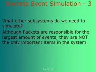
2. Discrete Event Simulation Is concerned with modelling of a system as it evolves over time by a representation in which the system variables change at discrete points on time Characteristics: • the passage of time is a part of simulation (Dynamic) • usually contains random elements (Stochastic)

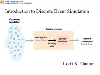
3. Discrete-Event Simulation Concepts • System: A collection of entities (e.g. people and machines) that interact together over time to accomplish one or more goals • Model: An abstract representation of a system, usually containing structural, logical, or mathematical relationships that describe a system in terms of its state, entities and their attributes, sets, processes, events, activities and delays. • System State: A collection of variables that contain all the information necessary to describe a system at any point in time

4. Discrete-Event Simulation Concepts • Entity: Any object or component in a system which requires explicit representation in the model (e.g. a server, a customer, a machine) • Attributes: Properties of a given entity (e.g. priority of a waiting customer, the routing number of a job through a job shop) • List: A collection of (permanently or temporarily) associated entities, ordered in some logical fashion (e.g. customers currently waiting in a queue ordered according to a queueing discipline) [sets, queues, chains]

5. Discrete-Event Simulation Concepts • Event: An instantaneous occurrence that changes the state of a system (e.g. arrival of a new customer) • Event Notice: A record of an event to occur at the current or some future time, along with any associated data to execute the event (at a minimum: event type, event time) • Event List: A list of event notices for future events, ordered by time of occurrence, also know as future event list (FEL)

6. Discrete-Event Simulation Concepts • Activity: A duration of time of specified length (e.g. service time), which is known when it begins. • deterministic • random • function of state variables or entity attributes (deterministic/random) • Delay: A duration of time of unspecified length, which is not directly known until it ends (an event triggers the end) [conditional wait] (e.g. time a customer spends in a waiting line) • Clock: A variable representing simulated time (CLOCK)

7. Events and System State A1 A2 S2 t2 t1 t3 t4 Time 0 S1 C1 C2 L(t) 2 1 0 t1 t2 t3 t4 Time B(t) 1 0 t1 t2 t3 t4 Time

8. Example: A Doctor’s Office

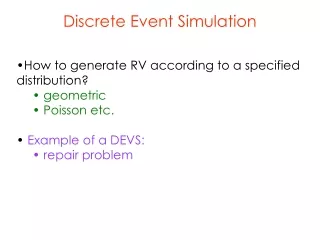
9. Example: A Doctor’s Office • System State • Q(t), the number of patients waiting to be examined at time t • B(t), 0 or 1 indicate the doctor being busy or not at time t • Entities • Neither the patients nor the doctor need to be explicitly represented, except in terms of state variables unless certain patient averages are desired • Events • Patient arrival event • Examination completion event

10. Example: A Doctor’s Office • Activities: • Interarrival time • Examination time • Delay • A patient’s wait until the doctor is free • What more to specify? • Consequences of events ( a logical description) • Activity lengths (deterministic, probabilistic, a function) • Triggers for the beginning and the end of delays • Initial conditions (System state at time 0)

11. Time Advance Advancing simulated time Variable time increments Fixed time increments Advances the clock to the most imminent event time & examine the system state Advances the clock by one time unit & examines the events and system state (ACTIVITY SCANNING) Approach Not an efficient approach for most systems EVENT ORIENTATION EVENT SCHEDULING NEXT EVENT METHOD

12. Variable Time Increment • Moves the system from one event time to the next event time • Produces a sequence of system snapshots (or system images) which represent the system evolution through time • System evolution can be represented by these snapshots since between events the system does not change

13. Variable Time Increment • Snapshots at each event time include: • The current state of the system • FEL for all activities currently in progress (their completion times) • The current membership to all lists • The status of all entities • Current values of all cumulative statistics and counters • Thus only the last snapshot is needed to construct the next snapshot (Markovian property)

14. Future Events List (FEL) • In real world, the future events are not scheduled but merely happen at a certain time (random arrivals, failures) • Yet these event times can be modeled by a statistical characterization (distribution) of the time to next occurrence (arrival, failure) • In simulation activity lengths are determined by obtaining a random sample from the distribution associated with it. • Completion Time = Starting Time + Activity Length • The activity completion time is determined as the activity begins and the activity completion event is added to FEL.

15. Event-Scheduling • At any given time t, the FEL contains all previously scheduled future events and their associated event times. • The FEL is ordered by event time, which means that the events are in chronological order. t < t1 <= t2 <= t3 <= . . . <= tn • The time t is the value of CLOCK, current value of simulated time • The event associated with time t1 is called the imminent event, which means the next event to occur. • The snapshot at CLOCK= t is updated

16. Event-Scheduling • Simulation time advances to CLOCK= t1 • Imminent event notice about t1 is removed from the FEL • The event is executed • The execution creates a new snapshot of the system at t1 based on the previous snapshot and the nature of the event • This snapshot may include new future event notices added to FEL or not(depends on the nature of the executed event) • And the cycle continues by repeating the same steps after advancing CLOCK to the time of the new imminent event until the end of the simulation

17. System Snapshot

18. System Snapshot

19. Future Event Generation • Exogenous Events (Events that are not caused by the internal dynamics of the system. They happen outside the system, yet effect the evolution of the system): • The events that are in the initial system snapshot at time 0 (specified by initial conditions). These are placed to the FEL before the simulation starts. • Other external events such as arrivals to a queueing system. These events are generated using a technique called Bootstrapping • This technique is based on each event causing another event of the same type • The time between the events is an activity (a) (It may be a r.v.) • When an event occurs, schedule the next event in the same stream of events and place the associated notice in the FEL • This next event in the stream is scheduled at t* = t + a

20. Bootstrapping

21. Future Event Generation • Endogenous Events • Service-completion event • Each time a customer starts service a service-completion event is scheduled (End of an activity) • Note that service-start event is never scheduled, it is called a conditional event. A service-start occurs within an arrival or a service-completion event. • The events that are placed on FEL are called primary events. • Uptimes and downtimes for a system subject to breakdown • End-of-uptime and end-of-downtime events (primary events) • Similar to bootstrapping

22. Stopping Simulation Runs • At time 0, schedule a stop-simulation event at a specified future time TE ( Simulation runs in the interval [0, TE] ) • Stop the run at the time of occurrence of some specified event E. (The completion of the 1000th service at the server)

23. World Views • When using a simulation package or even when doing hand simulation, a modeler adopts a world view or orientation for developing a model. • The most prevalent world views are • the event-scheduling world view • the process-interaction world view • the activity-scanning world view. • Particular simulation packages (e.g. Arena) usually support one of these world views.

24. Event-Scheduling World View • Concentrates on events and their effects on system state • It makes use of the Future Event List and variable time increments • This is the approach we have just discussed • It is a very flexible approach using which any system can be simulated • It requires lots of mechanisms (e.g. FEL handling) to be coded, which may slow down the development of the simulation model for very simple systems.

25. Event-Scheduling World View • We have not used this method on any example last week. We are going to do it now on the doctor’s office system • This is the world view that is usually used when the simulation program is directly coded on a general-purpose programming language such as Java. • We are going to show its implementation in Java next week • It would be hard to use this world view with EXCEL since the implementation of the standard mechanisms of Event-Scheduling is not easy in such environments (it could be done with extensive use of EXCEL macros)

26. Process-Interaction World View • Models the system in terms of processes • Concentrates on entities, and their life cycles as they flow through the system, demanding resources and queueing to wait for resources. • A process is a time-sequenced list of events, activities and delays that define the life cycle of one entity as it moves through a system. • Some activities might require resources that are limited, which may cause delays in the process

27. Process-Interaction World View • This is the world view we adopted for the hand simulation of the doctor’s office system last week

28. Process-Interaction World View • This approach is easier for the modeler since people usually perceive the systems in terms of the processes the entities experience • But this approach is usually harder to implement directly, especially when the systems to be simulated are complex • Thus, many simulation packages (including ARENA) use this view for the modeler to describe the system (user-interface), but an event-scheduling approach is used operationally to perform the simulation run, hidden from the user.

29. Activity-Scanning World View • Concentrates on activities and conditions that allow them to begin • It uses fixed time increments • At each clock advance, the conditions for each activity are checked, and if the conditions hold, then the corresponding activity starts. • The (M,N) inventory system simulation we used last week used activity-scanning approach. The time increment used was a day.

30. Activity-Scanning World View • Simple in concept and leads to modular models that are easier to maintain, understand and modify. • The repeated scanning (at each time increment) results in slow runtime on computers • The pure activity-scanning approach has been modified by what is called the three-phase approach, which combines the features of event-scheduling with activity scanning to allow for variable time advance. (ARENA uses this as well)

31. Example: A Doctor’s Office

32. Example: A Doctor’s Office • System State (Q(t),B(t)) • Q(t), the number of patients waiting to be examined at time t • B(t), 0 or 1 indicate the doctor being busy or not at time t • Entities • (Pi,t), representing patient Pi who arrived at time t • Events • Patient arrival event (A) • Patient departure event (D) • Stopping event (E)

33. Example: A Doctor’s Office • Event Notices • (A,t,Pi) represents the arrival of patient Pi at future time t • (D,t,Pi) represents the departure of patient Pi at future time t • (E,19) represents the simulation-stop event at future time 19 • Activities • Interarrival time, described in a following table • Service time, described in a following table • Delay • Patient time spent in the waiting room • Set • “Waiting Room”, the set of all patients in the waiting room • “Doctor’s Room”, the set of all patients in the doctor’s room

34. Arrival Event Arrival event occurs at CLOCK = t NO YES B(t)=1? B(t)=1 Q(t)=Q(t)+1 Generate service time s & schedule new departure event at t+s Generate interarrival time a; schedule next arrival event at t+a Collect statistics Return control to time-advance routine to continue simulation

35. Service Completion Event Departure event occurs at CLOCK = t Q(t) 1? NO YES B(t)=0 Q(t)=Q(t)-1 Generate service time s; schedule new departure at t+s Collect statistics Return control to time-advance routine to continue simulation

36. Input Data (Arrival) Interarrival time Probability Cumulative probability 1 0.30 0.30 2 0.25 0.55 3 0.20 0.75 4 0.15 0.90 5 0.07 0.97 6 0.03 1.00

37. Input Data (Service) Service time Probability Cumulative probability 1 0.25 0.25 2 0.25 0.50 3 0.25 0.75 4 0.25 1.00

38. Generation of interarrival times Interarrival time Cumulative probability Random digit assignment 1 0.30 01-30 2 0.25 31-55 3 0.20 56-75 4 0.15 76-90 5 0.07 91-97 6 0.03 97-00 Customer No. Random digit Interarrival time 1 - - 2 38 2 3 84 4 4 15 1 5 50 2 6 99 6 … … …

39. Generation of service times Interarrival time Cumulative probability Random digit assignment 1 0.25 01-25 2 0.25 26-50 3 0.25 51-75 4 0.25 76-90 Customer No. Random digit Service time 1 28 2 2 24 1 3 73 3 4 46 2 5 04 1 6 85 4 … … …

40. Statistics Continuous time statistics Discrete time statistics (Observational data) Time dependent data Continuous statistics Time weighted statistics Defined on the random variables {Q(t)},{B(t)}, each of which is indexed on the continuous time parameter Defined relative to the collection of random variables with a discrete time index (Observational data) ^

41. Notation TQ: time integral of Q(t) (from 0 to T) TB: time integral of B(t) (from 0 to T) TL: time integral of (B+Q)(t) (from 0 to T) R: total response time for patients (time-in-the-system) who departed by T W: total waiting time of patients (time-in-the-queue) who departed by T N: total number of departures by T Example: calculation of TL : TLnew=TLold+(T-Told)(Bold +Qold) T B+Q TL 0 1 0 2 1 0+(2-0)*1=2 3 0 2+(3-2)*1=3 6 1 3+(6-3)*0=3 19 13+(19-15)*1=17 0

42. Simulation table Clock B(t) Q(t) DR WR FEL R W N TQ TB 17 4 6 4 13

43. Machine (Server) Arriving Blank Parts Departing Finished Parts 7 6 5 4 Queue (FIFO) Part in Service Another Example of Hand Simulation using Event-SchedulingFrom Chapter 2 of the Arena Book

44. Model Specifics • Initially (time 0) empty and idle • Base time units: minutes • Input data (assume given for now …), in minutes: Part Number Arrival Time Interarrival Time Service Time 1 0.00 1.73 2.90 2 1.73 1.35 1.76 3 3.08 0.71 3.39 4 3.79 0.62 4.52 5 4.41 14.28 4.46 6 18.69 0.70 4.36 7 19.39 15.52 2.07 8 34.91 3.15 3.36 9 38.06 1.76 2.37 10 39.82 1.00 5.38 11 40.82 . . . . . . . . . . • Stop when 20 minutes of (simulated) time have passed

45. Simulation by Hand:Setup

46. Simulation by Hand:t = 0.00, Initialize

47. Simulation by Hand:t = 0.00, Arrival of Part 1 1

48. Simulation by Hand:t = 1.73, Arrival of Part 2 2 1

49. Simulation by Hand:t = 2.90, Departure of Part 1 2

50. Simulation by Hand:t = 3.08, Arrival of Part 3 3 2