Download
1 / 30
300 likes | 380 Vues
Dependent and Independent Samples. Problems. Problems. Confidence Interval – Dependent Samples Illustrative Problem. sample mean = 6.33 , Sx = 5.13, n = 6. Find the 95% confidence interval for the mean of the difference? (Sampling Distribution is t-distribution, 5df)

E N D
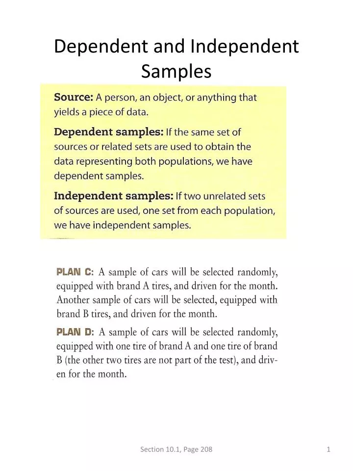
Dependent and Independent Samples Section 10.1, Page 208
Problems Problems, Page 230
Problems Problems, Page 230
Confidence Interval – Dependent SamplesIllustrative Problem sample mean = 6.33 , Sx = 5.13, n = 6 Find the 95% confidence interval for the mean of the difference? (Sampling Distribution is t-distribution, 5df) C.I. = sample mean ± Margin of Error = sample mean ± critical value * standard error 6.33 ± 2.5706 * 6.33 ± 5.38 = (.95, 11.71) Section 10.2, Page 211
Confidence Interval – Dependent SamplesIllustrative Problem TI-83 Black Box Program Find the 95% Confidence Interval d = B – A (We have to make the assumption that the data is taken from a normal population.) STAT – ENTER: Enter Brand A in L1 and B is L2 Highlight the title box for L3. =2nd L2 – 2nd L1 Enter (Difference set is now L3). STAT–TESTS- 8:TInterval Complete procedure as described in Section 9.1 Confidence Interval is (.96, 11.71) Section 10.2, Page 211
Hypothesis Test– Dependent SamplesIllustrative Problem sample mean = 6.33 , Sx = 5.13, n = 6 Test the hypotheses that the tread wear for Brand B is greater than for Brand A. Ho: μd = B – A =0 (No difference) Ha: μd = B – A > 0 (B is greater) p-value = .0146 μd=0 p-value = PRGM – TDIST LOWER BOUND = 6.33 UPPER BOUND = 2ND EE99 MEAN = 0 STANDARD ERROR = df = 5 Answer: p-value = .0147 (Reject Ho, B has greater tread wear.) Section 10.2, Page 211
Hypothesis Test– Dependent SamplesIllustrative Problem – TI-83 Black Box Program Test the hypotheses that the tread wear for Brand B is greater than for Brand A. (d=Brand B – Brand A) Ho: μd = 0 (No difference in wear) Ha: μd > 0 (Brand B has more wear) STAT – ENTER: Enter Brand A in L1 and B in L2 Highlight L3 =2nd L2 – 2nd L3 Enter (L3 in now difference set) STAT-TESTS– 2:T-Test Complete the program as described in Section 9.2 with L3 as the difference set. P-Value = .0146 (Reject H0, Brand B has greater tread wear.) Section 10.2, Page 211
Problems • Test the hypotheses that the people increased their knowledge. Use α=.05 and assume normality. State the appropriate hypotheses. • Find the p-value and state your conclusion. • Find the 90% confidence interval for the mean estimate of the increase in test scores. Problems, Page 231
Problems • State the appropriate hypotheses. • Find the p-value and state your conclusion. • Find the 98% confidence interval for the mean estimate of the increase in number of sit-ups. Problems, Page 232
Independent SamplesTwo Means: Unknown σ Suppose we want to compare the income of Shoreline students with UW students. From sample of 50 Shoreline Students: From sample of 60 UW students: Test the hypothesis that the populations incomes are not the same. To find a p-value we need a sampling distribution for Section 10.3, Page 215
Independent SamplesTwo Means: Unknown σ Population 1 Population 2 μ1 σ1 μ2 σ2 Sampling Dist. Sampling Dist. Sampling Dist. A T-Distribution Applies Section 10.3, Page 215
Independent SamplesTwo Means: Unknown σ • Conditions for t-distribution model for sampling distribution: • The samples are independent of each other – two unrelated sets of sources are used, one from each population. • The populations are normal, or the sample size from each population is large, n ≥ 30 The correct degrees of freedom for the sampling distribution for the difference of two independent means is given by the following formula: The calculator will make this calculation. Section 10.3, Page 215
Independent Means – Illustrative ProblemConfidence Interval – TI-83 Add-in Find the 95% confidence interval for the difference in the heights, μm – μf. C. I. = sample mean difference ± Margin of Error= sample mean difference ± critical value * standard error PRGM – STDERROR – 5: 2 MEANS Sx1 = 1.92; n1=30; Sx2 = 2.18; n2 = 20Answer: SE = .6004; df = 37.2121 PRGM – CRITVAL – 2 C – LEVEL = .95; df (INTEGER) = 37 Answer: 2.0262 C.I. = 69.8-63.8 ± 2.0262 * .6004 = (4.78, 7.22) Section 10.3, Page 216
Independent Means – Illustrative ProblemConfidence Interval – TI-83 Black Box Find the 95% confidence interval for the difference in the heights, μm – μf. STAT – TESTS – 0:2 – SampTInt Inpt: Stats : 69.8; Sx1: 1.92; n1: 30 : 63.8; Sx2: 2.18; n2: 20 C-Level: .95 Pooled: No Calculate Answer: (4.78, 7.22) Section 10.3, Page 216
Independent Means – Illustrative ProblemHypotheses Test– Add-In Programs Is this sufficient evidence to prove that male students are taller than female students. Ho: μm – μf = 0 μm = μf Ha: μm – μf > 0 μm > μf p-value ≅ 0 0 PRGMS – TDIST LOWER BOUND = 6 UPPER BOUND = 2ND EE99 MEAN = 0 STANDARD ERROR = .6004 (Slide 12) df = 37.2121 (Slide 13) Answer: p-value = 2.1930E-12 ≅ 0 (Reject Ho, there is sufficient evidence to prove males are taller.) Section 10.3, Page 216
Independent Means – Illustrative ProblemHypotheses Test– TI-83 Black Box Is this sufficient evidence to prove that male students are taller than female students. Ho: μm – μf = 0 μm = μf Ha: μm – μf > 0 μm > μf STAT – TESTS – 4: 2 – SampTTest Input: Stats :69.8; Sx1:1.92; n1:30 :63.8; Sx2:2.18; n2:20 μ1: >μ2 Pooled: No Calculate; Answer: p-value = 2.1947E-12≅0 (Reject Ho, there is sufficient evidence to prove males are taller) Section 10.3, Page 216
Problems • Write the necessary hypotheses. • State the p-value and your decision. • If you make an error, what type is it? • Construct a 98% confidence interval for the difference mean selling prices (North of Cedar – Provo) Problems, Page 233
Problems • Write the necessary hypotheses. • State the p-value and your decision. • If you make an error, what type is it? • Construct a 98% confidence interval for the difference mean weight gained (Diet B – Diet A) Problems, Page 233
Problems Assume normality. • Is there convincing evidence that nonorgan donors have higher anxiety about death than organ donors? Write the hypotheses and find the p-value. State your conclusion. • Find the mean and standard error of the sampling distribution. • Find the 98% confidence interval for the means; nondonor – donor. Problems, Page 232
Problems • State the hypothesis (Assume Normality) • Find the p-value, and state you conclusion. • Find the mean and standard error of the sampling distribution • Find the 95% confidence interval for the difference of the means; Gouda-Brie. Problems, Page 232
Independent SamplesTwo Proportions Suppose we want to compare the proportion of students getting financial aid at Shoreline and UW. From sample of 50 Shoreline Students: From sample of 60 UW students: Test the hypothesis that the population proportions are not the same. To find a p-value we need a sampling distribution for Section 10.3, Page 221
Independent SamplesTwo Proportions: Unknown σp Population 1 Population 2 p1 p2 Sampling Dist. p’1 Sampling Dist. p’2 Sampling Dist. p’1– p’2 The Normal Model Applies Section 10.4, Page 221
Two ProportionsConditions for Normal Model The sampling distribution for the difference of two sample proportions is a normal model if: Samples are independent of each other Each sample size > 20 Each sample has more than 5 successes (np or np’) and 5 failures (nq or nq’). (q=1-p) Each sample is not more than 10% of its population Section 10.4, Page 221
Two Proportions – Confidence Interval Illustrative Problem - TI-83 Add-In A campaign manager wants to estimate the difference in support between women and men for his candidate. A sample of 1000 for each population was taken, and 459 women and 388 men favored his candidate. Find the 99% confidence interval for pw – pm. C.I. = sample proportion difference ± Margin of Error = sample proportion difference ± critical value * standard error PRGM - CRITVAL – 1:NORMAL DIST – CONF LEVEL = .99 Answer: 2.5758 PRGM – STDERROR- 2: 2 PROP: p1 = 459/1000; n1 = 1000; p2 = 388/1000; n2 = 1000 Answer: sample proportion difference = .0710; standard error = .0220 C.I. = .0710 ± 2.5758*.0220 = (.0143, .1277) We are 99% confident that the proportion of female support exceeds the true proportion of male support is between 1.43% and 12.77%. Section 10.4, Page 222
Two Proportions – Confidence Interval Illustrative Problem - TI-83 TI-83 Black Box A campaign manager wants to estimate the difference in support between men and women for his candidate. A sample of 1000 for each population was taken, and 459 women and 388 men favored his candidate. Find the 99% confidence interval for pw – pm. STAT – TESTS – B:2PropZInt x1 = 459 n1= 1000 x2 = 388 n2 = 1000 C-Level = .99 Calculate Answer: (.0142, .1278) Section 10.4, Page 222
Difference between 2 Population Proportions For a hypothesis test, the null hypothesis is: Ho: p1 = p2. If the two proportions are equal, then the standard deviation of the proportions must be also equal. Since p’1 seldom equals p’2, the σ(p’1-p’2) does not reflect this fact. To get around this problem for hypothesis tests, we calculate the weighted average of p’1 and p’2, called p’p, or pooled sample proportion, and substitute is value for both p’1 and p’2 in the standard error calculation. Section 10.4, Page 223
Two Proportions – Hypotheses TestIllustrative Problem - TI-83 TI-83 Add-In A telephone salesman claims that his phones are better than the competition, and that no more of his phones are defective than the competition. A sample is taken. Can we reject the salesman’s claim? Use α = .05. Ho: ps = pc Ha: ps > pc PRGM – STDERROR – 3: 2-PROP POOLED p1 = 15/150; n1 = 150; p2 = 6/150; n2 = 150 Answer: p’s – p’c = .06; Standard Error = .0295 p-value = .0210 0 .06 PRGM – NORMDIST – 1 LB = .06; UB = 2nd EE99; MEAN = 0; SE( )= .0295 Answer: p-value = .0210. (Reject Null Hypotheses, and reject the salesman’s claim.) Section 10.4, Page 224
Two Proportions – Hypotheses TestIllustrative Problem - TI-83 TI-83 Black Box A telephone salesman claims that his phones are better than the competition, and that no more of his phones are defective than the competition. A sample is taken. Can we reject the salesman’s claim? Use α = .05. Ho: ps = pc Ha: ps > pc STAT – TESTS – 6:2PropZTest x1: 15 n1: 150 x2: 6 n2: 150 p1: >p2 Calculate Answer: p-value = .0208 (Reject the Null Hypotheses and the salesman’s claim.) Section 10.4, Page 224
Problems • Test the hypotheses that the preference in city A is greater than the preference in city B. State the appropriate hypotheses. • Find the p-value and state your conclusion. • What model is used for the sampling distribution and what is the mean of the sampling distribution and its standard error? • Find the 97% confidence interval for the difference in preferences, city A – city B. Problems, Page 235
Problems • State the appropriate hypotheses. • Find the p-value and state your conclusion. • What model is used for the sampling distribution and what is the mean of the sampling distribution and its standard error? • Find the 98% confidence interval for the difference in proportions, men – women. Problems, Page 234