Download

1 / 68
680 likes | 776 Vues
L.S.E.E.T. University Of Rhode Island. Recent progress in the modeling of non-linear free surface phenomena in ocean engineering. FRAUNIE, P. (1) GRILLI, S.T. (2) ;. L.S.E.E.T, Université de Toulon Department of Ocean Engineering, University Of Rhode Island.

E N D
L.S.E.E.T University Of Rhode Island Recent progress in the modeling of non-linear free surface phenomena in ocean engineering FRAUNIE, P. (1) GRILLI, S.T. (2) ; • L.S.E.E.T, Université de Toulon • Department of Ocean Engineering, University Of Rhode Island
WAVE BREAKING IN COASTAL ZONE • Objectives: • Coastal morphodynamics, sediment transport • Dammages on coastal areas and structures • Ocean-atmosphere interactions • Tools : • - Laboratory/in situ Experiments • - Numerical Simulation : Numerical wave tank Photos: www.pvergnaud.free.fr
Free surface flows • Flows containing several fluids/phases • Several examples : - wave breaking - cavitation - slushing of fuel in satellite tanks … better understanding of the physical phenomena • Tool : numerical simulation using interface tracking methods
t Fluid 1 Fluid 2 n Interface Assumptions : what is to be modeled ? • Flows : • Fully 3-D • Unsteady • Non hydrostatic • Laminar/turbulent • Single or two-phase flows • Fluids : • Newtonian • Incompressible or not
Mass conservation Velocity (m.s-1) Surface tension (N.m-3) Viscous stress tensor (N.m-2) r ì = div V 0 Pressure (N.m-2) r r í r r ¶ r r V ) t + r Ä - + Ñ = r + div ( V V ) P T î ¶ Body forces (m.s-2) Density (kg.m-3) Momentum conservation Mathematical formulation : conservation equations ï r ( f ï t … in the fluid domain
Fluid 1 Fluid 2 Interface Mathematical formulation : Interface boundary conditions Interface velocity Velocity continuity at the interface Normal to the interface Viscous fluids only Interface curvature Stress balance at the interface Surface tension coefficient
Mathematical formulation : boundary conditions • Solid boundaries : slip condition (Euler) or no-slip condition (Navier-Stokes), pressure extrapolation • Open boundaries : • - Dirichlet condition (fixed velocity and pressure) on inlet boundaries • - Neumann condition (normal derivative of the velocity imposed to zero) for the velocity and fixed pressure on outlet boundaries
Conservation equations Equation governing the interface evolution Interface conditions Boundary conditions C(x,t) = 1 if x fluid 1 C(x,t) = 0 if x fluid 2 Mathematical formulation : summary Resolve the system composed by: Equation governing the evolution of the interface Let be C the binary function so that :
Numerical resolution of the conservation equations : CFD code : EOLE (PRINCIPIA R&D) Navier-Stokes (or Euler) equations in a curvilinear formulation (ξ,η,χ) : F,G,H : flux terms (convective, diffusive, pressure) J : Jacobian of the transformation
Surface tension Body forces Numericalresolution ofthe conservation equations : With : • Space discretization : Centerred Finite Volume scheme (fields computed at the cell center) • Time discretization : second order implicit scheme
Pseudo-compressibility method (Chorin 1967) Concept : introduction of a time-like variable τ, the pseudo-time and of pseudo-unsteady terms New unknown introduced in the pseudo-unsteady terms, the pseudo-density Additional equation : pseudo equation of state giving the pressure as a function of the pseudo-density (Viviand):
Pseudo-compressibility method • Adding artificial viscosity terms avoids numerical oscillations • Integration step by step in pseudo-time thanks to a five step Runge-Kutta scheme (« dual time stepping ») Convergence : solution independent on τ corresponding to the numerical solution at time level n+1 Robust method allowing to deal with high density ratios
Time iteration pseudo-time iterations : pseudo time step calculation Runge-Kutta steps: flux computation, new velocity and pseudo-density, fixing the boundary conditions End of Runge-Kutta steps End of pseudo-time iterations Interface tracking method End of time iteration Algorithm :
extension of the SL-VOF method to 3-D flows Interface tracking method : aims • 3-D method allowing to deal with large deformations of the interface (large curvatures, reconnections, deconnections …) • Accuracy • Fast compared to classical V.O.F methods
Fluid 2 0.3 0.1 0 0.4 1 0.8 Fluid 1 1 1 0.9 b: values of C In each cell c: example of interface representation a : initial interface Volume Of Fluid (V.O.F) concept • The interface is tracked thanks to the volumic fraction of the denser fluid (fluid 1) : • C = 1 in a full cell of fluid 1 • C = 0 in a full cell of fluid 2 • 0 < C < 1 if a cell an interface occurs in the cell
V.O.F methods C function is advected with the fluids and verifies the transport equation : • Classical discretization schemes (centred, upwind, Quick …) are diffusing the interface and are not accurate • Alternative : methods with interface reconstruction. Several possibilities : • SOLAVOF method (Hirt & Nichols, 1981) • CIAM (Li, Zaleski, 1994) • SL-VOF (Guignard, 2001, Biausser 2003)
Interface reconstruction Interface advection Computation of the new V.O.F field SL-VOF 3-D method (B. Biausser, 2003) 3 steps allowing to update the interface during a time step :
(0,0,1) n (0,1,0) (0,0,0) (1,0,0) Step I : interfacereconstruction Piecewise Linear Interface Calculation (Li 1994) In each cell, the interface is represented by a plane portion (intersection of a plane with the computational cell) Interface
Step I : interfacereconstruction Two steps to calculate the interface plane portion : • Definition of the plane direction • Translation of the plane in order to verify the volume of the cell Calculation of the plane direction : the normal to the plane (orientated from denser the fluid towards the less dense fluid) is :
k k j j i i Step I : interfacereconstruction Evaluation of n by finite differences from the V.O.F of the neighbouring cells : a) Computation of normal vectors at the 8 corners of the cell: b) Normal vector is the mean of the 8 normal vectors at the corners
Step I : interface reconstruction Plane translation : the normal to the plane and the volumic fraction Cijk of the cell determine a unique plane Translation of the plane so that the volume contained under this plane is Cijk If the equation of the plane of normal nijk (nx, ny, nz) is nxx+nyy+nzz = , the problem is equivalent to calculate (Cijk,nijk)
Step I : interfacereconstruction The calculation of (Cijk,nijk) provides a unique plane portion : polygon from 3 to 6 sides whose corners are known B G A H (a) (b) (c) (d) (e) (f)
Interface after advection Xn+1 U.t Xn Interface before advection Step II : interface advection Calculation of the velocity at the polygon corners : bilinear interpolation from the velocities computed by the solver at the cell center Corners advection : first order (in time) Lagrangian scheme Xn+1 = Xn + U.t
Step II : interface advection After advection, the advected polygon corners are not necessarily coplanar so that a mean plane to these corners is defined : Normals to triangular subdivisions P3 Mean normal of the normals to triangulars subdivisions P4 Pm Polygon corners after advection P2 Mean point : iso-barycentre of the corners P1 Meanplane of the corners after advection (nm : mean normal , Pm : mean point) nm Pm
type B cells before advection Step III : computation of the new V.O.F field • Two configurations after advection : • Cells containing polygons portions (A type) • Cells without interface (B type) type A cells after advection
n1 n2 nm type A cellstreatment Calculation of the meanplane to all polygons parts in the cell : Mean plane defined by averaging the normals to the plane parts and their centres (weighted with the portions surface)
type A cellstreatment The new VOF of the cell is the volume generated by the averaged plane and is calculated by inversion of the formulae giving as a function of Cijk and nijk n New VOF : Cijkn+1
type B cells treatment • Two configurations are possible : • Cells loosing the interface during the time step : such cells become full (C = 1) or empty (C = 0) following the stream direction • Cells without interface before advection : the value of C remains the same Cell without interface before and after advection Cell filled up during advection
Evaluation of the method’s performances SL-VOF 3-D : summary • 3-D V.O.F. method with geometrical reconstruction of the interface • PLIC modeling (more precise than Hirt&Nichols) allowing to deal with large deformation of the interface • Lagrangian advection (possibly use of larger time steps than with classical methods)
Evaluation of the method’s performances • Comparison with a classical 3-D V.O.F method already developed in the EOLE code : FLUVOF (Hirt & Nichols kind) • Aability to deal with large changes of the interface • Ability to use large time steps
Comparison with FLUVOF 3-D • Comparison with a Hirt&Nichols method using a constant piecewise reconstruction of the interface (0 order) • Pure advection test-case (imposed velocity) : allows to test the methods performances without NS solver • Advection to a wall : the analytic velocity is known • A sphere advected in such a flow is progressively changed into ellipsoïds
Point A Solid wall 100 z x 0 100 Main direction of the flow Comparison with FLUVOF 3-D : computational domain In each transverse plane y = constant
Sphere advection in a distorting velocity field SL-VOF 3-D simulation
Comparison with FLUVOF 3-D Mesh 100X30X100
Comparison with FLUVOF 3-D • When the curvature is maximum, accuracy is better with SL-VOF 3-D than using FLUVOF : advantage of the P.L.I.Cdiscretization of the interface • The SL-VOF simulation is 4 times faster than FLUVOF : advantage of the Lagrangianadvection • Volume conservation is quite good : 0.13 % of loss compared to the initial fluid volume after 70 time steps The method’s approximates (mean plane) are not penalizing the volume conservation
Coupling with the NS solver : Rayleigh-Taylor instability • Stratified fluids of different densities (the denser is above) • Initial perturbation characteristic instability involving local vortices • Overturning of the interface occurs and the flow is computed with the full solver : good test for the method 2-D example (denser fluid in red)
Rayleigh-Taylorinstability • Density ratio: 2 • Perfect fluids in a cylindrical domain • Interface initially plane : sinusoidal perturbation of the velocity
Comparisons with 2-D axisymetric results 3-D on a radius 2-D axi
Tool able to deal with wave breaking Conclusions about the test cases • Compared to a classical V.O.F method : better accuracy when the curvature is increased, computational time is reduced • Large accurately deformations are taken into account
First tests of breaking Evaluation of the method’s ability to simulate wave breaking : • Breaking of an unstable linear wave • Breaking of a solitary wave on a beach of slope 1/15
Breaking of an unstable linear wave • Sinusoidal wave of high camber • Initial velocity field : Airy wave • Periodic boundary conditions over one wavelenght • L = 0.769 m • T = 0.86 s • D = 0.1 m • H = 0.1 m Fast evolving towards a plunging breaker
Propagation direction Déferlement d’une onde linéaire instable
Breaking of solitary waves on sloping beaches Conclusions concerning this test-case • Results comparable to those of Abadie (1998) on the same test-case for 2-D flows (aspect of the breaker jet, splash-up, maximal velocity about 2 times the phase celerity) • First simulation of breaking conclusive with the method (reconnections and deconnections of the interface, curvature …) • Artificial breaking, generated by a non-physical initial condition
Breaking on a beach of slope 1/15 • Solitary wave H0 = 0.5 m • Computational domain : flat bottom and then sloping bottom • Initialisation with Tanaka’s algorithm (1986) and computation of the initial fields with Boundary Integral Equations Method of S. Grilli : potential code using a Boundary Element Method
Boundary Integral Equations Method • Nonlinear potential flows with a free surface • Fast and accurate method for wave shoaling and overturning applications • Unable to deal with breaking (no reconnection, irrotationnal and inviscid flows …)