Download
1 / 19
190 likes | 347 Vues
Co-Design Implementation of a System for Model Predictive Control. P. Vouzis 1 , L. Bleris 2 , M. V. Kothare 3 & M. Arnold 1 1 Computer Engineering 2 Electrical Engineering 3 Chemical Engineering Lehigh University. 2005 AIChE Annual Meeting. d. Reference. u(k). y(k). Plant. MPC.

E N D
Co-Design Implementation of a System for Model Predictive Control P. Vouzis1, L. Bleris2, M. V. Kothare3 & M. Arnold1 1Computer Engineering 2Electrical Engineering 3Chemical Engineering Lehigh University 2005 AIChE Annual Meeting
d Reference u(k) y(k) Plant MPC u(k) Model Predictive Control (MPC) • Model Predictive Control • Use a predictive model of the plant • Step-wise decision with look ahead prediction • Flexibility on the control objectives past target future Projected outputs Manipulated variable u(k+l),l=0,1,…,m-1 k k+1 k+m-1 k+p-1 control horizon m prediction horizon p
Computational Issues in MPC • MPC relies on the solution of an optimization problem by minimizing a cost function: • Complexity:n = (# inputs) × (control horizon) • Abundant matrix operations for real-time implementations s.t.: Bar[m]<U[m]<Bar[m] B = P×M A = P×N Yref = 1×M P:Prediction Horizon M:Control Horizon N: Number of states Newton’s optimization algorithm requires the calculation of:
Need for Embedded MPC • MPC is proven technology for advanced optimal control in chemical process industry • Advantages • Can handle MIMO systems • Can handle constraints explicitly • Can handle uncertainties and disturbances • Can handle nonlinearities • Restricted to systems with slow dynamics • Requires dedicated computer Clear need/opportunity to embed MPC in hardware for high-speed size-constrained control problems
Applications of Embedded MPC • Drug Delivery • Robotics • Microfluidic control • Educational Platform for Academia
Desired Properties • Low-power consumption • Small size • Limited memory (~300 Kb) • High speed • Efficient implementation of matrix multiplication, inversion • Fast memory access • Reliable • Low-cost
Previous Work • Parametric studies to relate precision to control performance – proposed ASIC design Bleris, L. G., M. V. Kothare, J. G. Garcia and M. G. Arnold. Towards Embedded Model Predictive Control for System-on-a-Chip Applications. To appear: Journal of Process Control, 2005. • Off-the-self processor implementation Bleris, L. G. and M. V. Kothare.Implementation of Model Predictive Control for Glucose Regulation using a General Purpose Microprocessor. In: 44th IEEE Conference on Decision and Control and European Control Conference. Seville, Spain, 2005.
Input (16 bits) 16-bit µP Core Matrix Coprocessor + LNS Output (16 bits) Write Read CS Data or Status Proposed Approach Codesign General Purpose µP Matrix Coprocessor
Logarithmic Number System (LNS) • In LNS a number X is represented by its logarithmic value: x=log(X) • Multiplication and division in LNS simplified: • log(X×Y)=log(X)+log(Y)=x+y • log(X/Y)=log(X)-log(Y)=x-y • …but addition and subtraction are more difficult: • log(X+Y)=max(x,y)+log(1+2|x-y|)) • log(X-Y)=max(x,y)+log(1-2|x-y|) Storing the two functions is the most costly part for implementing the LNS
What is co-design • Co-Design offers the combination of increased HW performance and the flexibility of SW
Case Study: Antenna Rotation • Rotate the antenna so that it follows a moving object in the plane • -2 V < u< 2 V
Percentage of total time Control Horizons HW-SW Partitioning • Gradient, Hessian, Gauss-Jordan Matrix Coprocessor • Newton, Initialization General purpose µP
Matrix Initialization for (int i = 0; i < M; i++) for (int j = 0; j< M; j++){ if(i==j) A[i][j]=1.0; else A[i][j]=0.0 } Matrix Addition for (int i = 0; i < M; i++) for (int j = 0; j< M; j++) A[i][j] += m[i][j]; Matrix Multiplication for (int i = 0; i < M; i++) for (int j = 0; j< M; j++) { A[i][j]=0.0; for (int k = 0; k < P; k++) A[i][j] += A[k][i]*C[k][j]; } (The matrices are sent only initially to the Coprocessor and invoked only when necessary) Matrix Initialization SEND=STORE_IDENT_A Matrix Addition SEND=ADD_A SEND=Memory_location Matrix Multiplication SEND=MUL_C SEND = Memory_location Software Simplification with Coprocessor Stand-alone µP Software µP software w/ Coprocessor Finally the coupled uP-Coprocessor system will be a flexible platform to implement different algorithms that require matrix manipulation
Input (16 bits) 16-bit µP Core Matrix Coprocessor + LNS Output (16 bits) Write Read CS Data or Status Hardware in the Loop (HIL) Simulation • HIL simulation: interface the developed system with a host that can simulate real-world operating conditions Plant Set point u(k) y(k) _ • Real world conditions are achieved without the actual risk of using a real device with a system under development • The system can be simulated under extreme conditions that is difficult to be reproduced only for testing purposes • Parts of the system can be tested before having the complete design ready
HIL Simulation Outputs 5 optimization iterations Red → controlling voltage Blue → angular position Black → set point Magenta → constraint
HIL Simulation Outputs 10 optimization iterations Red → controlling voltage Blue → angular position Black → set point Magenta → constraint
Implementation Overview • µP used: ADCUS SE1608 16 bit • FPGA used: Virtex IV of Xilinx • Development environment: ISE 7.1 of Xilinx & EISC Studio of ADCUS
Conclusions • Co-design approach proposed • Optimal partitioning of operations between HW and SW based on profiling results • Coprocessor and LNS architecture proposed • First systematic effort to integrate real-time optimal predictive control with HW level implementation issues
Acknowledgements • U.S. National Science Foundation ("XYZ-on-Chip" initiative, CAREER) • Pittsburgh Digital Greenhouse • ADC Inc. (U.S.A.) hardware platform