Atmospheric Science 8600 Advanced Dynamic Climatology

1. Atmospheric Science 8600 Advanced Dynamic Climatology Anthony R. Lupo 302 E ABNR Building Department of Soil, Environmental, and Atmospheric Science University of Missouri Columbia, MO 65211 Phone: 573-884-1638 Email: LupoA@missouri.edu Web.missouri.edu/~lupoa/atms8600.html or atms8600.pptx

2. ATMS 8600 Dynamic Climatology • Syllabus ** • 1. Introductory and Background Material for ATMS 8600. • 2. Define Climate and climate change. • 3. The Equations of climate processes • 4. Physical processes involved in the maintenance of climate.

3. ATMS 8600 Dynamic Climatology • 5. Climate Modelling, a history and the present tools. • 6. Climate Variations: Past climates and what controls climate? • 7. Climate change: Inductive and deductive theories. • 8. Climate and Climate change (natural vs. “anthropogenic”, what is the current conventional wisdom?) • ** Students with special needs are encouraged to schedule an appointment with me as soon as possible!

4. ATMS 8600 Dynamic Climatology • This class will essentially just go 'upscale' from ATMS 8400 - Theory of the General Circulation. • Some initial questions: • What is Climate? How does it differ from weather (synoptic, or even the General Circulation)? How is this different from Climatology? • Weather  the day to day state of the atmosphere. Includes state variables (T, p) and descriptive material such as cloud cover and precipitation amount and type, etc.

5. ATMS 8600 Dynamic Climatology • Recall in meteorology, we tend to divide phenomena by scale based on what processes are important to driving them. • Table 1

6. ATMS 8600 Dynamic Climatology • General Circulation – ‘statistical’ features. We think of planetary in scale, but time scales are 2 weeks, 1 month, 1 season, 1 year, a few years. • Climate Is the long-term or time mean state of the Earth-Atms. system and the state variables along with higher order statistics. Also, we must describe extremes and recurrence frequencies. • Thus, the general definition of climate is scale independent and a technical definition would depend on your scale, ie we can describe micro, meso, and synoptic climates and climatologies. • Climate as we will discuss it many contexts will be "global" or large-scale in nature, or "upscale" in time from the General Circulation.

7. ATMS 8600 Dynamic Climatology • Climatology is the study of climate in a mainly descriptive and a statistical sense. Climatologists study these issues. • Dynamic Climatology or Climate dynamics are relatively new concepts and involve the study of climate in a theoretical and/or numerical sense. In order to study climate in this sense, we will use models, which will be derived using basic equations. • One way to accomplish this is via the scaling of primitive equations, or using basic 'RT' equations (Energy Models, which use concepts like Stefan Boltzman'slaw).

8. ATMS 8600 Dynamic Climatology • Key concepts that will be discussed in this course: • We'll need to distinguish plainly between weather and climate! (Review the concept of climatic averaging') • We'll need to talk about time variations on climate states ('climate' versus climate change) • We'll need to examine the components of the climate system

9. ATMS 8600 Dynamic Climatology • We'll need to examine the state of the climate, in particular this means 'internal variables' (internal vs. external). • We'll need to study climatic 'forcing' (this means 'external variables (e.g. Solar, Plate tectonics, humans?), (also how they differ from internal)) • We'll need to examine issues surrounding spatial resolution and climatic character.

10. ATMS 8600 Dynamic Climatology • The primary components of the Climate system • 1. The Atmosphere (typical response time --> minutes to three weeks) • 2. The Ocean (typical response time months and years, for upper ocean) • 3. The litho-biosphere (we'll treat as one for now) • 4. The cryosphere (both land and sea ice, response times on order of decades to MYs)

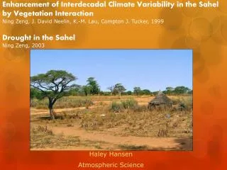
11. ATMS 8600 Dynamic Climatology • The earth-atmosphere system, courtesy of Dr. Richard Rood. (http://aoss.engin.umich.edu/class/aoss605/lectures/)

12. ATMS 8600 Dynamic Climatology • Aside: • Typical short-hand notations used now in the study of climate: • 10,000 Years Before present (10 KY BP) KY = Thousands of years BP = before present • MY = Millions of years.

13. ATMS 8600 Dynamic Climatology • Another view of the climate system

14. ATMS 8600 Dynamic Climatology • Another view

15. ATMS 8600 Dynamic Climatology • Each component of the climate system can be described by it's own state variables, which are considered internal variables. • External forcing is defined as forcing outside the system or sub-system. Thus, SST anomalies are internal or state variables for the earth atmosphere system, or the ocean. But they are considered 'forcing' or external to the atmospheric component. • Also, the dynamics of the internals are fairly well know, but heat and mass exchange processes between sub-sytems not well understood.

16. ATMS 8600 Dynamic Climatology • Ok, now we have to introduce ourselves to the concept of climatic averaging. • For any instantaneous climatic variable a; • a (bar) representing a time mean, and a' the instantaneous departure from the mean.

17. ATMS 8600 Dynamic Climatology • Recall, that (from mean value theorem): • where t' will represent a 'dummy' time coordinate, and t is physical time, and t is the averaging time usually written as =t . For the above to be valid in a physical sense, then: • P(a') <<  << P(a)

18. ATMS 8600 Dynamic Climatology • where P(a) represents a characteristic time period, say a few seconds for wind gusts (P(a')?), and 3 - 4 days for an extratropical cyclone (P(a)?)

19. ATMS 8600 Dynamic Climatology • In drawing on the previous slide, I've provided for you a CLEAR separation between the two periodic fluctuations. • In the climate system one must look for periods of high and low variability, to do this we can look at an idealized (not real) periodogram for the atmosphere. • Periodogram(real) examines the "power" spectrum within a time series of say, Temperature. "power" or variance is the square of the Fourier coefficients:

20. ATMS 8600 Dynamic Climatology • An idealized Temperature Spectrum for Earth

21. ATMS 8600 Dynamic Climatology • This spectrum demonstrates 'scale' separations nicely (planetary, synoptic, meso, micro): • typical averaging periods: example: 1 sec, 1 hr, 3-12 mo., 30 years, 1 MY • Turbulence  way out on right • 'weather' and gen circ. 12 hr to 1 yr typically. • climate (as is commonly thought of) is 1 yr to 27 year peak. • climate change scale: 30 yrs to 100 KYs. • tectonic change: on left.

22. ATMS 8600 Dynamic Climatology • Forcing: • External forcing Is “boundary value” forcing. These are independent of the system and can be altered externally. These refer to forcing outside the system or outside the sub-system is it is closed. Example: solar radiation. • Internal forcing are forcings that operate within the system and can arise out of non-linear interactions within a system. Example: Vorticity advection, temperature advection, latent heating.

23. ATMS 8600 Dynamic Climatology • The State of the Climate System • In the climate system can be considered a composite system, if as a whole the system is thermodynamically closed (impermeable to mass, but not energy), (recall from gen circ., we say mass does not change). • The individual sub-components are thermodynamically open (transfers of mass and energy allowed) and cascading (that is the output of mass or energy from one subsystem becomes the input into another). • The state of the climate system can be represented in terms of physical variables that represented additive of extensive properties (e.g., volume or internal energy, or angular momentum), or in terms of intensive properties ('fields') that are independent of total mass and that change with time ('temperature', pressure, and wind velocity).

24. ATMS 8600 Dynamic Climatology • Equilibration of the Climate System • If for specific time scales, the internal climate system behaves as if it has forgotten its past, and responds primarily to external forcing then it can be considered to be almost in the state of equilibration. • External forcing can be outside earth atmosphere. system, or be forcing from an internal variable of longer time-response (inertial time scale) sub-systems forcing on another sub-system (e.g. SST forcing) with a shorter time response. (e.g., if considering synoptic-scale, then ice sheets, oceans, and everything is 'external').

25. ATMS 8600 Dynamic Climatology • Thus the climate system is a boundary value problem, this is different from weather forecasting with is primarily an initial value problem (boundaries there too). These definitions allow us to define climate in terms of ensemble means and variability of each sub-system independently. • If any initial state always leads to the same near equilibrium climatic state (same equilibrium properties), then the system is transitive (climate folks) or ergodic (geology folks!).

26. ATMS 8600 Dynamic Climatology • Transitive (weather forecasts, “cycles” diurnal and annual)

27. ATMS 8600 Dynamic Climatology • If instead there are two or more different states with different properties that result from different initial conditions, then the system is intransitive (this system – stochastic, dynamic laws unknown - pack it up and go home w/r/t forecasting). • If there are different subsets of statistical properties, which a transitive system assumes during its evolution from different initial states, through long but finite periods of time, the system is almost intransitive. • In this case, the climate state, beginning from any initial condition will always converge to the same state eventually, but go through periods w/ distinctly different climatic regimes. This is best representation of climate system. (Ice ages?)

28. ATMS 8600 Dynamic Climatology • Intransitivity (weather forecasts) and “almost intransitive” (oscillations);

29. ATMS 8600 Dynamic Climatology • Concept: Diagnostic vs. Prognostic • Quick definition: prognostic equations have a on the Left hand side • Diagnostic equations have no time derivatives. • Example: Equation of state (ideal gas law).

30. ATMS 8600 Dynamic Climatology • A more precise (correct) definition: sourcesink • This is a standard ordinary differential equation, or Forced – Dissipative equation/system. This is nothing new.

31. ATMS 8600 Dynamic Climatology • F = any external forcing (source) •  = damping constant (sink) • This is one way to view long-term climate change. • If  < =  (damping is large, strong or instantaneous) we have a diagnostic, or equilibrium problem such that (the two RHS terms cancel or nearly so;

32. ATMS 8600 Dynamic Climatology • If  >>  and  >= P(a) then we have a prognostic equation or non-equilibrium problem, e.g., • These properties allow us to distinguish based on approximate values of (), fast response variables is diagnostic and slow response variables are prognostic variables in climate system.

33. ATMS 8600 Dynamic Climatology • For climate: • fast response (diagnostic)  atmosphere • slow response (prognostic)  ice sheets, ocean • (for example, if ice sheets grow, we know how atmosphere will behave)

34. ATMS 8600 Dynamic Climatology • Diagnostic or prognostic?

35. ATMS 8600 Dynamic Climatology • Climate Modeling • Definition of a Climate Model: • An hypothesis (frequently in the form of mathematical statements) that describes some process or processes we think are physically important for the climate and/or climatic change, with the physical consistency of the model formulation and the agreement w/ observations serving to 'test' the hypothesis (i.e., the model). • "The model (math) should be shortened (approximated) for testing the hypothesis, and the model should jive with reality".

36. ATMS 8600 Dynamic Climatology • The scientific Method: • 1. Collect Data • 2. Investigate the Issue • 3. Identify the Problem • 4. Form Hypothesis • 5. Test Hypothesis • 6. Accept or Reject hypothesis based on conclusions • 7. If reject, goto 2 • 8. If accept, move on to the next problem.

37. ATMS 8600 Dynamic Climatology • Two distinct types of climate models: • 1) Diagnostic or equilibrium model (Equilibrium Climate Model - ECM) with time derivatives either implicitly or explicitly set to zero. The ECM is most commonly solved for climatic means and variances. (d / dt = Force + Dissipation) • 2) Prognostic models, where time derivatives are crucial and with the variation with time of particular variables the desired result (i.e., a time series). Most commonly solved for changes in climatic means and variances. Weather models (General Circulation Models – GCMs)

38. ATMS 8600 Dynamic Climatology • Ocean - Atmosphere (one of many subsystems of the climate system) • (go back to our diagram) • Some basic principles: • Conservation of mass  precipitation, evaporation: precip= evap over the globe (closed system). Water vapor budget equation we also use in Atms 8400. • Energy: Sun heats land and oceans which, in turn, heats the atmosphere (transparent to shortwave, but opaque to LW). • In order to fully understand, we should couple the atmosphere - ocean is more important than considering each separately, however, we know each separately!

39. ATMS 8600 Dynamic Climatology • Feedback Mechanisms • Feedback mechanisms complicate things, Nature is highly non-linear. But they are a good way to get a handle on non-linear coupling mechanisms. • Feedback mechanisms are all positive (+) or negative (-) • (+) amplify the linear response to a forcing process. (e.g., ice-albedo) – indicate a “sensitive” system. • (-) de-amplify the response to a forcing process. (e.g., clouds – global temperature)

40. ATMS 8600 Dynamic Climatology • Examples: Double CO2 • -Positive feedback- • Linearly increase CO2 to double the amount has a very small effect on climate temp. response or forcing. • It's the other feedbacks that amplify "global warming" • CO2is a "potent" greenhouse gas, but a trace gas.

41. ATMS 8600 Dynamic Climatology • Water Vapor is more plentiful and 30 times more potent "greenhouse gas" (molecule per molecule, due to vibrational, rotational absorption bands). • Increased CO2, (could) mean increased water vapor. This increases the long wave retained by atmosphere, which heats up atmosphere and oceans. (IPCC) • Increased water vapor  increased LW heating,  increased evaporation  increased water vapor. (Get the picture? Positive feedback!). This will go on forever, unless something interrupts. • Caveat: Increases in air temp, does not necessarily mean corresponding increases in specific humidity and dew points. • Formula for + feedback: E happens A inc B incC incA inc.

42. ATMS 8600 Dynamic Climatology • -- negative feedback -- • Clouds again same caveat, more vapor not necessarily means more clouds, and consider cloud characteristics, like droplets, or ice crystals, drop size, optical depth, etc. • More low clouds, increases Earth's albedo, less SW into the system, LW out exceeds SW in and cooling. • May dampen a positive feedback, bring the system back into equilibrium, but not necessarily at the same state that was the original. • Formula - feedback: E happens A inc.B inc.C incA dec.

43. ATMS 8600 Dynamic Climatology • Temperature measurements and records (problems w/ climate data) • Must make objective (homogeneous)! • Climate statistics there are large imhomogenetiesin time and space for recorded measurements (station moved?, instrumentation changed? obs. practices changed? land surface change?). These are hard to get a handle on in reality? Does observation match reality? • Many problems exist! • "to make these records homogeneous, we have to choose an objective weighting scheme". However, choice is highly objective!! Skeptics can see no change, proponents can see change

44. ATMS 8600 Dynamic Climatology • How do we generate such records? Past Variations of Climate! • 1. What do we really mean? • 2. How do we reconstruct past climates? • 3. How do we infer past variations in climate? • 4. Types of climatic data? • In order to "see" past climate you must understand present!

45. ATMS 8600 Dynamic Climatology • 3 types of climate data • Observed observed data, there is about 350 years for England, 200 years in the West, 15 to 50 years globally. • Historical based on historical recordings, diaries, paintings, etc. Most is qualitative and uncertain, but we have this back 100's to 1000's of years. • Proxy infer climate, via chemical biological, and sediment records.

46. ATMS 8600 Dynamic Climatology • Typically proxy records involve examining pollen/spore records in sediment or fossils, and/or matching plant and animal species with current climate types. • We can also infer climate from isotope records, for example examining Carbon-13 or Oxygen-18 isotopes. Plant different plant species use C-13 differentially, thus it is easy to tell what species persisted in some area by examining remains. • O-18. There is more O-18 in the oceans under colder climes (the molecules less likely to evaporation than lighter ones). • Read the two articles about proxy determination. The approach is largely statistical, i.e. we correlate concentrations to Tavg's and come up with a regressive relationship.

47. ATMS 8600 Dynamic Climatology • Also read (Pollen): • Woodhouse, C.A., and J.T. Overpeck, 1998: 2000 years of drought variability in the Central United States. Bull. Amer. Met. Soc., 79, 2693 - 2714.

48. ATMS 8600 Dynamic Climatology • The Fundamental Equations: • Now my favorite part - the equations. Not only will we examine these in a climate sense, but we will examine for a general substance, (fluid) as well. Think of this as 'fluid dynamics' • What we are doing is representing (or evaluating) meteorological, oceanographic, or other relevant observations. Since these observations are taken at discrete intervals of time (say about 6 hrs for weather observations), we assume synoptically averages conditions. That is: • x = X + X* (synoptic mean and dep.) • The equations we'll derive will be general then climatologically avg'd.

49. ATMS 8600 Dynamic Climatology • Recall our general conservation laws: • 1) Cons. of Mass (vol.) Continuity (Water mass also!) • 2) Cons. of momentum (N-S equations) • 3) Cons. of Energy (1st law) • and don't forget elemental kinetic theory of gasses (State (constituent) variable relationships) • Continuity: • Notation c = carrier fluid a = atms. w = ocean i = ice j = trace constituents

50. ATMS 8600 Dynamic Climatology • Xc = mass concentration of carrier fluid • Xj = mass conc. of jth trace constituent • Total density of an arbitrary volume in the climate system • Often times, Xc >> Xj