Download
1 / 41
410 likes | 415 Vues
Progress on Technical Work to Support Haze SIPs. Planning and Policy Group Colorado APCD October 11, 2007. Content of Presentation- Ray- this slide is just a guide taken from the notes from Tom- Look at comment section below.

E N D
Progress on Technical Work to Support Haze SIPs Planning and Policy Group Colorado APCD October 11, 2007
Content of Presentation- Ray- this slide is just a guide taken from the notes from Tom- Look at comment section below • Please describe how you are presenting technical support documentation for your Haze Plan. • 1) Provide an example of how you obtained, analyzed, and documented technical data about 2000-04 baseline and 2064 natural conditions, glide paths for deciviews and individual species, source types, source regions, et cetera? • 2) Provide an example of how you analyzed emissions and developed 2000-04 baseline and 2018 projection emissions budgets for sources in your state. a. What is the projected change in controllable emissions by species? b. What are the uncontrollable sources by species, and how large are they? • 3) What analyses and documentation have you made of sources contributing to haze at your Class I area(s) that are out of your state's control, i.e., other states' emissions, international impacts from Off-shore shipping, Mexico, Canada, the rest of the world? • 4) What kinds of future regional technical work is needed to better understand impacts at Class I areas in your state especially if current analysis of strategies shows only modest showing little or modest visibility improvement?
Topics for Presentation • Colorado SIP schedule • SIP development • Technical Support Document and related efforts
SIP Schedule • Hearing initially scheduled for November but extended by one month to address the “Four Factors” and other matters • Once Plan approved by Air Commission, legislative approval still needed
SIP Development • Last minute plan elements being drafted now (our deadline is the 26th of October) • Major chunks still being developed including “Four Factors” and EPA and FLM comments on BART determinations
How Colorado has and is presenting technical support documentation for your Haze Plan • Technical Support Document developed for each Class I area • All TSDs are on the Division’s Regional Haze homepage • Four Workshops for stakeholders and our target audience • Web site with frequent updates
Topic 1: Defining the 2000-04 baseline and 2064 natural conditions, glide paths for deciviews and individual species, source types, source regions From the Technical Support Document and the workshops… • Section 3 – Visibility Conditions • Section 4 – Haze impacting particles – best and worst days • Section 5-6 – Inventories and modeling
Colorado Regional HazeState Implementation Plan DevelopmentPublic Hearing I September 21, 2006 Colorado Air Quality Control Commission Presented by: Dan Ely and Curt Taipale
Page 11 IMPROVE History • IMPROVE = • Interagency Monitoring of Protected Visual Environments • IMPROVE monitoring network was established in 1985 • To measure visibility impairment at Class I areas • Funded by EPA • Monitoring began in 1988 at 30 monitoring sites. • For RH rule the network had 110 sites by 2001 • 156 Class I areas and 110 monitoring sites • Not all Class I Areas have monitors but ALL have representative monitoring
Page 12 Access to IMPROVE Data • VIEWS (Visibility Information Exchange Web System) web site: • http://vista.cira.colostate.edu/views/ • Sponsored by all RPOs, but created by the WRAP • Processed data in the form of graphics are available • Trend data are also available
Page 13 Graphical Data
Page 14 Division Recommendations Comments/Questions? • IMPROVE Equations • Division Recommends using the new IMPROVE equation • Rationale: Better represents extinction, based on recent science, and consistent with Regional Modeling
Page 15 Baseline & Natural Conditions • Determining Baseline Conditions • Determining Natural Conditions • Default Natural Conditions • Natural Haze Levels II
Page 16 Baseline Conditions • Baseline Conditions • Represent visibility for the 20% best and 20% worst days over a 5-year period extending through calendar year 2000-2004. • The Best and Worst Baseline Conditions are the starting points for EPA’s 60 year RH program. • No degradation of best days • Reasonable progress to 2064 goal on worst days • Baseline values are determined by: • Best days: calculate the average deciview value for the 20% best days for each of the 5 years (2000-2004) and then average those five values to arrive at one overall baseline average. • Worst days: Same procedure for the worst days.
Page 17 Great Sand Dunes National Park & PreserveEstablished as National Monument in 1932, National Park in 2000 84,600 acres The Sangre de Cristo Mountains loft over the great dunes (Photo courtesy of NPS)
Page 20 Species-Specific Uniform Progress
Provide an example of how you analyzed emissions and developed 2000-04 baseline and 2018 projection emissions for sources in your state. a. What is the projected change in controllable emissions by species? b. What are the uncontrollable sources by species, and how large are they?
Colorado Regional Haze SIP Reasonable Progress Analysis Rocky Mountain National Park Longs Peak – 14,259’ Colorado’s 15th Tallest
Page 24 Analysis Context • Time is short – SIPs are due in December • Ideally, today’s Reasonable Progress analysis should be based on final BART modeling for the whole WRAP region • Realistically, it’s too late to implement additional controls beyond BART • In lieu of these limitations, Colorado plans “State Share” analysis for determining RP on the dominant man-caused species of visibility impairing pollutants – sulfate & nitrate • Assumes that each state is working on emission reduction strategies that benefit all impacted Class I Areas • Some CIAs w/high out-of-state impacts may not benefit from this approach • Can be addressed through interstate collaboration • OC addressed with limited PSAT; EC, CM & fine soil can be addressed through a more basic analysis using weighted emission potential (WEP), emission inventory (EI), positive matrix factorization (PMF) and Emissions Trace (ET) • Analysis focused on Worst Days • Assume 2018 model projections are adequate for estimating maintenance of Best Days • Future IMPROVE monitoring will validate this assumption
Page 25 Measure Progress from Glide Slope • In the extinction metric, 23% is not the goal for each species, 2018 modeling progress is measured against the URP point on glide slope. • Non-linearity between extinction and HI is addressed by the curve of the extinction glide slope. • For ROMO, the corresponding 2018 extinction reduction is about 28%
Page 26 Preliminary 2018 Modeling Results(three RRFs methods averaged)
What analyses and documentation have you made of sources contributing to haze at your Class I area(s) that are out of your state's control, i.e., other states' emissions, international impacts from Off-shore shipping, Mexico, Canada, the rest of the world?
Page 28 4-Highest Sulfate & Nitrate Contributors at ROMO • We see that Boundary Conditions are the highest contributor for SO4 and 2nd for NO3 at Rocky in 2018. • Across Colorado, BCs are the highest sulfate contributor for all our CIAs and in the top 3 for nitrate.
What is the Emissions Trace? • Tool that graphically organizes and prioritizes a vast of array of visibility & emissions information from the WRAP • Specific to each IMPROVE Monitor • Looks at 20% Worst Days • Specific to each visibility impairing pollutant • Sulfate, Nitrate, OC, EC, Soil and Coarse Mass • Attribution of Natural/Anthropogenic Sources • Primary/Secondary Aerosols • PM Source Apportionment Technology (PSAT) • Boundary Conditions, International, WRAP States, Other RPOs & Colorado Share • Weighted Emissions Potential (WEP) • Emissions Inventory
Understanding the ET • Read from left to right • Top bar (purple) denotes general source of information • Colors denote different types particulates/sources • Lt Green: secondary particulate from natural sources • Lt Yellow: primary particulate from anthro/natural sources • Lt Blue: secondary particulate from anthropogenic sources • Gray color bars provide specific detail on source of data • WEP map provides information on likely source areas
ROMO Sulfate - ET • ROMO has highest monitored Sulfate concentrations (~24%) in State Source Categories 2,000 tpy are identified as significant
Page 32 ROMO 2018 Sulfate Emissions Trace
ROMO Sulfate PSAT • Sulfate PSAT – full apportionment of all states/regions • About 94% of sulfate is anthropogenic on worst days • WRAP ~50% (Colorado <24%), Outside Model Domain ~30%, CENRAP ~7%, remaining 13% mostly from international areas • Colorado Point Sources are the dominant source category
Colorado Point Source SO2 Significant Point Source Categories
Colorado Area Source SO2 Significant Area Source Categories
Controlling ROMO Sulfate • Colorado Point Sources (~18% or 69,345 tpy of SO2) • External Combustion Boilers – 519 in category • Coal-fired Boilers are largest category • About 21 sources emit 61,517 tpy of SO2 emissions • Some existing sources have SO2 controls and some BART sources are adding SO2 controls • Industrial Processes – 3147 in category • Chemical Products, Mineral Products & Petroleum Production largest • Top 25 emit 5,412 tpy of SO2 emissions • Colorado Area Sources (~3% or 7,395 tpy of SO2) • Boilers & IC Engines are largest category • Distillate fueled • Colorado Mobile Sources (~1% or 938 tpy of SO2) • From diesel-fueled engines
Page 37 ROMO 2018 Nitrate Emissions Trace
Page 38 Top Colorado NOx Point Sources • BART controlled sources highlighted in green • Closest big non-BART NOx source • Rawhide (285 MW) has LNB w/OFA
Summary of ROMO OC, EC, Soil & CM • Visibility Impact ~32% but over 70% natural - wildfire • CO share ~17.2% (see OC-ET) • Area ~61%, Rx Fire ~19%, Mobile ~18% • Meaningful reductions unlikely (e.g.- 50% control of above <3%) • Visibility Impact <8% and CO Share ~76% • Wildfire ~42%, Mobile ~22%, Area ~11% • Meaningful reductions unlikely (e.g.- 50% control of M&A <1%) • Visibility Impact ~4% and CO Share ~45% • Fugitive Dust ~20%, Area ~14%, Mobile ~6%, Wildfire ~5% • Meaningful reductions unlikely (e.g.- 50% control of M&A <1/2%) • Visibility Impact ~15.1% and CO Share ~46% • Fugitive Dust ~21%, Point ~17%, Road Dust ~4%, Wildfire ~2% • Meaningful reductions unlikely (e.g.- 50% control of P&RD <1%)
What kinds of future regional technical work is needed to better understand impacts at Class I areas in your state especially if current analysis of strategies shows only modest showing little or modest visibility improvement?
Next Steps • Division to initiate a “Reasonable Progress” stakeholder process in 2008 • Goal to develop a “RP” rule that can be used to evaluate potential emission control strategies for significant source categories.