Download

1 / 70
700 likes | 703 Vues
TESTS FOR NOMINAL SCALEDATA : CHI-SQUARE TEST. OBJECTIVE. In this lecture, you will learn the following items: How to perform a chi-square goodness-of-it test. How to perform a chi-square test for independence. INTRODUCTION.

E N D
OBJECTIVE In this lecture, you will learn the following items: • How to perform a chi-square goodness-of-it test. • How to perform a chi-square test for independence.
INTRODUCTION Sometimes, data are best collected or conveyed nominally or categorically. These data are represented by counting the number of times a particular event or condition occurs. In such cases, you may be seeking to determine if a given set of counts, or frequencies, statistically matches some known, or expected, set. Or, you may wish to determine if two or more categories are statistically independent. In either case, we can use a nonparametric procedure to analyze nominal data. In this lecture, we present three procedures for examining nominal data: chi square (2) goodness of it, 2-test for independence, and the Fisher exact test.
THE χ2 GOODNESS-OF-FIT TEST • Some situations in research involve investigations and questions about relative frequencies and proportions for a distribution. • Some examples might include a comparison of the number of women pediatricians with the number of men pediatricians, a search for significant changes in the proportion of students entering a writing contest over 5 years, or an analysis of customer preference of three candy bar choices. • Each of these examples asks a question about a proportion in the population.
Computing the χ2 Goodness-of-Fit Test Statistic • The χ2 goodness-of-it test is used to determine how well the obtained sample pro- portions or frequencies for a distribution it the population proportions or frequencies specified in the null hypothesis. • The χ2 statistic can be used when two or more categories are involved in the comparison. Formula 1 is referred to as Pearson’s χ2 and is used to determine the χ2 statistic:
where fo is the observed frequency (the data) and fe is the expected frequency (the hypothesis). Use Formula 2 to determine the expected frequency fe: Use Formula 3 to determine the degrees of freedom for the χ2 -test: where C is the number of categories.
Example • χ2 Goodness-of-Fit Test • (Category Frequencies Equal) A marketing firm is conducting a study to determine if there is a significant preference for a type of chicken that is served as a fast food. The target group is college students. It is assumed that there is no preference when the study is started. The types of food that are being compared are chicken sandwich, chicken strips, chicken nuggets, and chicken taco. The sample size for this study was n = 60. The data in Table 1 represent the observed frequencies for the 60 participants who were surveyed at the fast food restaurants.
We want to determine if there is any preference for one of the four chicken fast foods that were purchased to eat by the college students. Since the data only need to be classified into categories, and no sample mean nor sum of squares needs to be calculated, the χ2 statistic goodness-of-it test can be used to test the nonparametric data.
1. State the Null and Research Hypotheses The null hypothesis states that there is no preference among the different categories. There is an equal proportion or frequency of participants selecting each type of fast food that uses chicken. The research hypothesis states that one or more of the chicken fast foods is preferred over the others by the college student. The null hypothesis is: HO: In the population of college students, there is no preference of one chicken fast food over any other.
HA: In the population of college students, there is at least one chicken fast food preferred over the others. Thus, the four fast food types are selected equally often and the population distribution has the proportions shown in Table 2.
2. Set the Level of Risk (or the Level of Significance) Associated with the Null Hypothesis
3. Choose the Appropriate Test Statistic The data are obtained from 60 college students who eat fast food chicken. Each student was asked which of the four chicken types of food he or she purchased to eat and the result was tallied under the corresponding category type. The final data consisted of frequencies for each of the four types of chicken fast foods. These categorical data, which are represented by frequencies or proportions, are analyzed using the χ2 goodness-of-it test.
4. Compute the Test Statistic First, tally the observed frequencies, fo, for the 60 students who were in the study. Use these data to create the observed frequency table shown in Table 3.
Table 4 presents the expected frequencies for each category.
5. Determine the Value Needed for Rejection of the Null Hypothesis Using the Appropriate Table of Critical Values for the Particular Statistic Before we go to the table of critical values, we must determine the degrees of freedom, df. In this example, there are four categories, C = 4. To find the degrees of freedom, use df = C − 1 = 4 − 1. Therefore, df = 3.
6. Compare the Obtained Value with the Critical Value The critical value for rejecting the null hypothesis is 7.81 and the obtained value is χ2 = 13.21. If the critical value is less than or equal to the obtained value, we must reject the null hypothesis. If instead, the critical value exceeds the obtained value, we do not reject the null hypothesis. Since the critical value is less than our obtained value, we must reject the null hypothesis. Note that the critical value for = 0.01 is 11.34. Since the obtained value is 13.21, a value greater than 11.34, the data indicate that the results are highly significant.
7. Interpret the Results We rejected the null hypothesis, suggesting that there is a real difference among chicken fast food choices preferred by college students. In particular, the data show that a larger portion of the students preferred the chicken strips and only a few of them preferred the chicken taco.
8. Reporting the Results The reporting of results for the χ2 goodness of it should include such information as the total number of participants in the sample and the number that were classified in each category. In some cases, bar graphs are good methods of presenting the data. In addition, include the 2 statistic, degrees of freedom, and p-value’s relation to . For this study, the number of students who ate each type of chicken fast food should be noted either in a table or plotted on a bar graph. The probability, p < 0.01, should also be indicated with the data to show the degree of significance of the χ2.
For this example, 60 college students were surveyed to determine which fast food type of chicken they purchased to eat. The four choices were chicken sandwich, chicken strips, chicken nuggets, and chicken taco. Student choices were 10, 25, 18, and 7, respectively. The χ2 goodness-of-it test was significant: (χ2(3) =13.21, p < 0.01). Based on these results, a larger portion of the students preferred the chicken strips while only a few students preferred the chicken taco.
Example χ2 Goodness-of-Fit Test (Category Frequencies Not Equal) Sometimes, research is being conducted in an area where there is a basis for different expected frequencies in each category. In this case, the null hypothesis will indicate different frequencies for each of the categories according to the expected values. These values are usually obtained from previous data that were collected in similar studies.
In this study, a school system uses three different physical fitness programs because of scheduling requirements. A researcher is studying the effect of the programs on 10th-grade students’ 1-mile run performance. Three different physical fitness programs were used by the school system and will be described later.
Using students who participated in all three programs, the researcher is comparing these programs based on student performances on the 1-mile run. The researcher recorded the program in which each student received the most benefit. Two hundred fifty students had participated in all three programs. The results for all of the students are recorded in Table 5.
We want to determine if the frequency distribution in the case earlier is different from previous studies. Since the data only need to be classified into categories, and no sample mean or sum of squares needs to be calculated, the χ2 goodness-of-it test can be used to test the nonparametric data.
1. State the Null and Research Hypotheses The null hypothesis states the proportion of students who benefited most from one of the three programs based on a previous study. As shown in Table 8.6, there are unequal expected frequencies for the null hypothesis. The research hypothesis states that there is at least one of the three categories that will have a different proportion or frequency than those identified in the null hypothesis.
The hypothesis is: HO: The proportions do not differ from the previously determined proportions shown in Table 6. HA: The population distribution has a different shape than that specified in the null hypothesis.
2. Set the Level of Risk (or the Level of Significance) Associated with the Null Hypothesis
3. Choose the Appropriate Test Statistic The data are being obtained from the 1-mile run performance of 250 10th-grade students who participated in a school system’s three health and physical education programs. Each student was categorized based on the plan in which he or she benefited most. The final data consisted of frequencies for each of the three plans. These categorical data which are represented by frequencies or proportions are analyzed using the χ2 goodness-of-it test.
Compute the Test Statistic First, tally the observed frequencies for the 250 students who were in the study. This was performed by the researcher. Use the data to create the observed frequency table shown in Table 7.
Table 8 presents the expected frequencies for each category.
7. Interpret the Results We rejected the null hypothesis, suggesting that there is a real difference in how the health and physical education program affects the performance of students on the 1-mile run as compared with the existing research. By comparing the expected frequencies of the past study and those obtained in the current study, it can be noted that the results from program 2 did not change. Program 2 was least effective in both cases, with no difference between the two. Program 1 became more effective and program 3 became less effective.
It is often a good idea to present a bar graph to display the observed and expected frequencies from the study. For this study, the probability, p < 0.01, should also be indicated with the data to show the degree of significance of the χ2.
For this example, 250 10th-grade students participated in three different health and physical education programs. Using 1-mile run performance, students’ program of greatest benefit was compared with the results from past research. The χ2 goodness-of-it test was significant (χ2(2)=19 08, p < 0.01). Based on these results, program 2 was least effective in both cases, with no difference between the two. Program 1 became more effective and program 3 became less effective.
THE χ2TEST FOR INDEPENDENCE Some research involves investigations of frequencies of statistical associations of two categorical attributes. Examples might include a sample of men and women who bought a pair of shoes or a shirt. The first attribute, A, is the gender of the shopper with two possible categories:
The second attribute, B, is the clothing type purchased by each individual:
We will assume that each person purchased only one item, either a pair of shoes or a shirt. The entire set of data is then arranged into a joint-frequency distribution table. Each individual is classified into one category which is identified by a pair of categorical attributes (see Table 9).
The χ2 -test for independence uses sample data to test the hypothesis that there is no statistical association between two categories. In this case, whether there is a significant association between the gender of the purchaser and the type of clothing purchased. The test determines how well the sample proportions it the proportions specified in the null hypothesis.
1. Computing the χ2 Test for Independence The χ2 -test for independence is used to determine whether there is a statistical association between two categorical attributes. The χ2 statistic can be used when two or more categories are involved for two attributes. Formula 4 is referred to as Pearson’s χ2 and is used to determine the χ2 statistic:
In tests for independence, the expected frequency fejk in any cell is found bymultiplying the row total times the column total and dividing the product by thegrand total N. Use Formula 5 to determine the expected frequency fejk: The degrees of freedom df for the χ2 is found using Formula 6: where R is the number of rows and C is the number of columns.
It is important to note that Pearson’s χ2 formula returns a value that is too small when data form a 2 × 2 contingency table. This increases the chance of a type I error. In such a circumstance, one might use the Yates’s continuity correction shown in Formula 7:
Daniel (1990) has cited a number of criticisms to the Yates’s continuity correction. While he recognizes that the procedure has been frequently used, he also observes a decline in its popularity. Toward the end of this course, we present an alternative for analyzing a 2 × 2 contingency table using the Fisher exact test.
Where χ2 is the chi-square test statistic and n is the number in the entire sample.
Example χ2 Test for Independence A counseling department for a school system is conducting a study to investigate the association between children’s attendance in public and private preschool and their behavior in the kindergarten classroom. It is the researcher’s desire to see if there is any positive association between early exposure to learning and behavior in the classroom.