Download
1 / 61
620 likes | 738 Vues
Descriptive Statistics, Histograms, and Normal Approximations. Math 1680. Overview. Obtaining Data Sets Descriptive Statistics Histograms The Normal Curve Standardization Normal Approximation Summary. Obtaining Data Sets. Before we can analyze a data set, we need to have a data set

E N D
Descriptive Statistics, Histograms, and Normal Approximations Math 1680
Overview • Obtaining Data Sets • Descriptive Statistics • Histograms • The Normal Curve • Standardization • Normal Approximation • Summary
Obtaining Data Sets • Before we can analyze a data set, we need to have a data set • How far do you travel to get to class, in miles? • How tall are you? • Today, numerical data is easily stored and organized (and even analyzed) by several computer programs
Obtaining Data Sets • Notice that in its raw form, the data is difficult to deal with • By sorting the data, we can get a better picture of its distribution, or shape • We are often interested in… • Where the data are centered • How spread out they are • With what frequency numbers appear
Obtaining Data Sets • Usually, the entire data set is too large to work with directly • We want ways to summarize the data • We have quantitative (numerical) and pictorial descriptions available to us • Descriptive Statistics • Histograms
Descriptive Statistics • We can summarize the data set with a few simple numbers, called descriptive (or summary) statistics • The first and most often-used summary stat is the average (or mean) • Represents the central tendency of the data set • Gives an idea of where the bulk of the points lie • To calculate the average, add up the values of all of the points and divide by the total number of points in the set
Descriptive Statistics • Calculate the average of the following data sets • 60 60 60 60 60 • 18 59 60 63 100 • 18 35 60 87 100
Descriptive Statistics • Despite having the same average, the three data sets are clearly different • The average alone usually does not describe data sets uniquely
Descriptive Statistics • The median is another central tendency measure • The median marks the point where exactly half of the data are less than (or equal to) the median • If there are an odd number of data points, then the median is just the number in the middle of the sorted set • Otherwise, the median is the average of the two points in the middle of the sorted set
Descriptive Statistics • Calculate the median of each data set • 1 4 5 7 10 15 18
Descriptive Statistics • The average is like a balance point • It represents the place where the data set is equally “heavy” on both sides • If there are outliers on one side of the data set, the average will be skewed • The median is more robust • What this means is that it is usually less s affected by outliers or data entry errors.
Descriptive Statistics • In a certain class of 13 students, 10 showed up the first exam, while 3 blew it off • Here are the grades; in order: • Calculate the class median… • Including all students • Not counting those who slept in 79 82.5
Descriptive Statistics • In a certain class of 13 students, 10 showed up the first exam, while 3 blew it off • Here are the grades; in order: • Calculate the class average… • Including all students • Not counting those who slept in 62.8 81.7
Descriptive Statistics • Suppose the teacher mistyped the grade of 55 as being a 15 • Not counting the sleepers, • What is the new median? • What is the new average? 82.5 77.7
Descriptive Statistics • Earlier, we saw that the average did not necessarily uniquely describe a data set • We use the standard deviation (SD) to measure spread in a data set • When paired, the average and SD are highly effective summary statistics
Descriptive Statistics • The Root-Mean-Square (RMS) measures the typical absolute value of data points in a set • Calculated by reading its name backwards • Square all entries in the data set • Take their mean • Take the square root of that mean • Find the average and then the RMS size of the numbers of the list Average = 0 RMS = 4
Descriptive Statistics • The SD embodies the same concept of “typical” distance • Where the RMS measures typical distance from 0, the SD measures typical distance from the data set’s average • This is accomplished by subtracting the average from every data point and then taking the RMS of the differences (or deviations from the mean)
Descriptive Statistics • 1 4 5 7 10 15 has an average of 7 • The deviations are then -6 -3 -2 0 3 8 • Note how the subtraction process re-centers the data set so that the average is at 0
Descriptive Statistics • Taking the RMS of the deviations gives the standard deviation • Normally, about two thirds to three quarters of a data set should be within one SD of the mean • 1 4 5 7 10 15 has an average of 7 and an SD of about 4.5
Descriptive Statistics 1 4 5 7 10 15 (1+4+5+7+10+15)/6 = 7 Average = 7 1-7 4-7 5-7 7-7 10-7 15-7 -6 -3 -2 0 3 8 (-6)2 (-3)2 (-2)2 02 32 82 (36+9+4+0+9+64)/6 = 122/6 ≈ 20.3 √(20.3) ≈ 4.5 36 9 4 0 9 64 SD ≈ 4.5
Descriptive Statistics • What we had on the previous slide is called the SD of the sample. However, if the goal is to use this sample to estimate the SD of a larger population, we would divide by n-1 instead of n (where n is the number of points) and call the result Sample SD. • Most calculators actually calculate the sample SD. • In general, the higher a set’s SD, the more spread out its points are • An SD of 0 indicates that every point in the data set has the same value
Descriptive Statistics • Calculate the SD’s of the data sets • 60 60 60 60 60 • 18 59 60 63 100 • 12 35 60 87 100 0 26.0 30.7
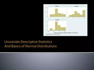
Histograms • Often, we would prefer a pictorial representation of a data set to a two-number summary • The most common way to graphically represent a data set is to draw a frequency histogram (or just histogram)
Histograms • Histograms tend to look like city skylines • In a histogram, the area under the curve between two points on the horizontal axis represents the proportion of data points between those two points • Continuing the city skyline analogy, the size of the building determines how many people live there • A long, low building can house as many people as a thin skyscraper
Histograms • To draw a histogram, we first need to organize our data into bins (or class intervals) • Often, the bins are dictated to us • If we get to choose them, we try to pick the bins so that they give a fair representation of the data • Then mark a horizontal axis with the bin values, spacing them correctly
Histograms • Often, data is given in percentage form • If not, divide the number of points in the bin by the number of points in the data set to get the percentage • Draw a box for each bin so that the area of the box is the percentage of the data in that bin • To get the correct height of the box, divide the percentage of the box by the width of the bin
Histograms • Note that the average and median can be visually located on a histogram • If the histogram was balanced on a see-saw, the fulcrum would meet the histogram at the average • If you draw a vertical line through the histogram so that it splits the area in half, then the line passes through the median • On a symmetric histogram, the average and median tend to coincide • Asymmetric tails pull the average in the direction of the tail
The Normal Curve • A great many data sets have similarly-shaped histograms • SAT scores • Attendance at baseball games • Battery life • Cash flow of a bank • Heights of adult males/females
The Normal Curve • These histograms are similar to one generated by a very special distribution • It is called the normal distribution, and it is identified by two parameters we are already familiar with • average • standard deviation
The Normal Curve • This is the standard normal curve, where the average is 0 and the SD is 1
The Normal Curve • Though the equation used to draw the curve is not easy to work with, there is a table of values for the standard normal distribution • We will use this table to find areas under the curve • The table is on page A-105 of your text
The Normal Curve • Properties of the standard normal curve • The curve is “bell-shaped” with its highest point at 0 • It is symmetric about a vertical line through 0 • The curve approaches the horizontal axis, but the curve and the horizontal axis never meet
The Normal Curve • Area underneath the standard normal curve • Half the area lies to the left of 0; half lies to the right • Approximately 68% of the area lies between –1 and 1 • Approximately 95% of the area lies between –2 and 2 • Approximately 99.7% of the area lies between –3 and 3
Standardization • Most data sets do not have a mean of 0 and an SD of 1 • To be able to use the standard normal curve, we’ll need to standardize numbers in the original data set • To standardize a number, subtract the data set’s average and then divide the difference by the data set’s SD • Standardizing is basically a change of scale • Like converting feet to miles
Standardization • Suppose there are two different sections of the same course • The scores for the midterm in each section were approximately normally distributed • In first section, the average was 64 and the standard deviation was 5 • Tina scored a 74 in first section • In second section, the average was 72 and the standard deviation was 10 • Jack scored an 82 in second section • Which of the two scores is most impressive, relative to the students in his/her section?
Standardization • Convert the following scores in the first section to standard units • Alice got a 50 • Bob got a 61 • Carol got a 64 • Dan got a 77 -2.8 -0.6 0 2.6
Standardization • In Jack’s section, students with grades between 62 and 82 received a B • What percentage of students in this section received Bs? • Is this percentage exact? 68.27% No
Normal Approximation • According to the HANES study, the height of U.S. women was 63.5 inches with an SD of 2.5 inches
Normal Approximation • The normal curve is a smooth-curve histogram for normally distributed data • We can estimate percentages within a given range • Find the area under the curve between those ranges using the standard normal table
Normal Approximation • Sometimes will require cutting and pasting different areas together • The standard normal table on page A-105 takes a standard score z • It returns to you the area under the curve between –z and z
Normal Approximation • Find the area between –1.2 and 1.2 under normal curve 76.99%
Normal Approximation • Find the area between 0 and 1.65 under the standard normal curve 45.055%
Normal Approximation • Find the area between 0 and 3.3 under the standard normal curve 49.9515%
Normal Approximation • Find the area between –0.35 and 0.95 under normal curve 46.58%
Normal Approximation • Find the area between 1.2 and 1.85 under the normal curve 8.29%
Normal Approximation • Find the area between –2.1 and –1.05 under the normal curve 12.9%
Normal Approximation • Find the area to the right of 1 under the normal curve 15.865%
Normal Approximation • Find the area to the left of 0.85 under the normal curve 80.235%
Normal Approximation • If a data set is approximately normal in distribution, we can use the normal curve in place of the data set’s histogram • If you want to estimate the percentage of the data set between two numbers… • Standardize the numbers to get z scores • Look each z score up in the standard normal table • Cut and paste the areas to match the region you originally wanted • The percentage under the curve will be close to the percentage in the data set