Download
1 / 18
200 likes | 589 Vues
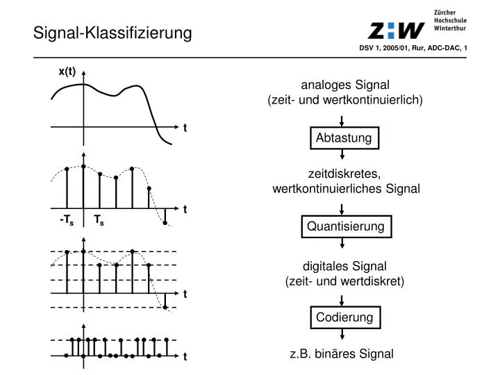
Signal-Klassifizierung. DSV 1, 2005/01, Rur, ADC-DAC, 1. x(t). analoges Signal (zeit- und wertkontinuierlich). t. Abtastung. zeitdiskretes, wertkontinuierliches Signal. t. -T s. T s. Quantisierung. digitales Signal (zeit- und wertdiskret). t. Codierung. z.B. binäres Signal. t.

E N D
Signal-Klassifizierung DSV 1, 2005/01, Rur, ADC-DAC, 1 x(t) analoges Signal (zeit- und wertkontinuierlich) t Abtastung zeitdiskretes, wertkontinuierliches Signal t -Ts Ts Quantisierung digitales Signal (zeit- und wertdiskret) t Codierung z.B. binäres Signal t
Natural Sampling und ideale Abtastung DSV 1, 2005/01, Rur, ADC-DAC, 2 x(t) t = nTs T0 T0 t t T0 -Ts Ts t -Ts Ts xs(t) x(t) t = nTs t t -Ts Ts t -Ts Ts
Zeitbereich x(t) xs(t) = x(nTs) = x[n] Frequenzbereich 1. Nyquistzone … … 2. Nyquistzone 2. Nyquistzone Ts·Xs(f) -fs fs Spektrum abgetastetes cos-Signal DSV 1, 2005/01, Rur, ADC-DAC, 3
SHA im ADC DSV 1, 2005/01, Rur, ADC-DAC, 4 sampling clock Timing analoger Input ADC Encoder digitaler Output S track (S zu) hold (S offen) track (S zu)
Aliasing und Rekonstruktion DSV 1, 2005/01, Rur, ADC-DAC, 5 X(f) f fg Fall fs>2fg Xs(f) Spiegelspektren (Images) HTP(f) f - fs - 3fs - 2fs fs 2fs 3fs Fall fs<2fg Xs(f) Aliasing f - 2fs - fs - 3fs - 4fs fs 2fs 3fs 4fs
Digitalisierungssystem DSV 1, 2005/01, Rur, ADC-DAC, 6 fs fs fg < fs/2 fg < fs/2 DAC mit ZOH* „DSP“ ADC ZOH- Kompensation* Anti-Aliasing- Filter H(f) Post-Filter* * Komponenten Rekonstruktionsfilter IH(f)I Durchlass- bereich Übergangs- bereich Sperr- bereich DR DR f fs fg fs-fg fs/2
Idealer Rekonstruktions-Tiefpass DSV 1, 2005/01, Rur, ADC-DAC, 7 Frequenzbereich H(f) Normierte Frequenz f / fs Zeitbereich Ts· h(t) Normierte Zeit t · fs
Ideale Rekonstruktion (Zeitbereich) DSV 1, 2005/01, Rur, ADC-DAC, 8 rekonstruiertes Signal x(t) ideal abgetastetes Signal xs(t) idealer TP fg=fs/2 Interpolationsfunktionen x(Ts) x(t) = cos(2π(fs/16)t) t Ts
Zero-Order-Hold am DAC-Ausgang DSV 1, 2005/01, Rur, ADC-DAC, 9 hZOH(t) 1 t Ts Amplitudengang ZOH-Filter -14 dB -4 dB (kompensierbar) Postfilter
Visualisierung Abtastung + Rekonstruktion DSV 1, 2006/01, Hrt, ADC-DAC, 10
Undersampling DSV 1, 2005/01, Rur, ADC-DAC, 11 Abtastung Basisbandsignal 1. Nyquistzone 2. Nyquistzone 3. Nyquistzone 4. Nyquistzone Original Image Image Image f fs 2fs Abtastung BP-Signal in ungerader Nyquistzone Image Original Image Image f fs 2fs Abtastung BP-Signal in gerader Nyquistzone (Kehrlage) Image Original Image Image f fs 2fs
Quantisierungskennlinie DSV 1, 2005/01, Rur, ADC-DAC, 12 xq(nTs) 011 3Δ 010 2Δ out of range 001 Δ 000 x(nTs) -4Δ Δ/2 Δ 2Δ 3Δ -3Δ -2Δ -Δ 111 -Δ 110 out of range -2Δ x(nTs) xq(nTs) Quantisierer 101 -3Δ 100 x(nTs) xq(nTs) -4Δ ε(nTs)
Aperture und Clock Sampling Jitter DSV 1, 2005/01, Rur, ADC-DAC, 13 ∆xrms x(t) Schalter offen (hold) track track t tj SNR = -20·log10(2πf·tj)
DDS: Einsatzbeispiel DSV 1, 2005/10, Rur, ADC-DAC, 14 Zeitbereich Frequenzbereich S(f) f Verschiebung s(t) y(t) Y(f) cos(2πf0t) f0 einstellbar (DDS) f -f0 f0 Y(f) = 0.5·S(f-f0) + 0.5·S(f+f0)
DDS: Grundprinzip DSV 1, 2005/10, Rur, ADC-DAC, 15 Lookup-Tabelle mit N Werten einer Sinus-Periode t 0 Ts=1/fs DAC (ZOH) TP fs Phase[n] = (Phase[n-1] + M) mod N (Phase entspricht Adresse) f0 = M·fs/N t T0 0 Ts=1/fs Fall M=2 t 0 Ts=1/fs
DDS: Blockdiagramm DSV 1, 2005/10, Rur, ADC-DAC, 16 seriell oder parallel Vref Tuning-Wort M truncation w = 24-48 Bits w 12-19 Bit 10-14 Bit Sinus Lookup- Tabelle w Phasenregister DAC TP w Phasen-Akkumulator DDS-Baustein (NCO) Referenz-Clock fs (fs ≤ 25…1000 MHz, je nach Baustein)
DDS: Spektrum DSV 1, 2005/10, Rur, ADC-DAC, 17 analoges TP-Filter 0 dB -4 dB Kopien SFDR 2 2 „Rauschen“ f [MHz] f0=30 fs/2=50 70 fs=100 130
DDS: Eigenschaften DSV 1, 2005/10, Rur, ADC-DAC, 18 schnelles und flexibles Frequenztuning neuen M-Wert seriell oder parallel laden und frei schalten sehr hohe Frequenzauflösung Beispiel AD9834: fs=50 MHz, 28-Bit Tuning-Wort => Δf < 0.186 Hz spektrale Reinheit genügt vielen Anwendungen SFDR-Werte im Bereich 60-90 dB kontinuierliche Phase Frequenzwechsel ohne Phasensprung oder mit definierter Startphase Frequenz- und Phasenumtastung (FSK/PSK) FSK: Umtasten zwischen 2 Tuning-Wörtern M0 und M1 Sweeping und Frequency Hopping (FH) FH: automatische, periodische Aktivierung verschiedener M-Werte relativ hoher Stromverbrauch Leistungsaufnahme steigt mit Abtastfrequenz stark an relativ hoher rms-Jitterwert als Clock-Signal für schnelle ADCs ungeeignet


![[Unix Programming] Signal and Signal Processing](https://cdn3.slideserve.com/5708599/unix-programming-signal-and-signal-processing-dt.jpg)