Download

1 / 38
400 likes | 491 Vues
Influence matrix diagnostic to monitor the assimilation system Carla Cardinali. ECMWF 4D-Var system handles a large variety of space and surface-based observations. It combines observations and atmospheric state a priori information by using a linearized and non-linear forecast model.

E N D
Influence matrix diagnostic to monitor the assimilation systemCarla Cardinali
ECMWF 4D-Var system handles a large variety of space and surface-based observations. It combines observations and atmospheric state a priori information by using a linearized and non-linear forecast model Monitoring Assimilation System • Effective monitoring of a such complex system with 108 degree of freedom and 107observations is a necessity. No just few indicators but a more complex set of measures to answer questions like • How much influent are the observations in the analysis? • How much influence is given to the a priori information? • How much does the estimate depend on one single influential obs?
Diagnostic methods are available for monitoring multiple regression analysis to provide protection against distortion by anomalous data Influence Matrix: Introduction • Unusual or influential data points are not necessarily bad observations but they may contain some of most interesting sample information • In Ordinary Least-Square the information is quantitatively available in the Influence Matrix Tuckey 63, Hoaglin and Welsch 78, Velleman and Welsch 81
The OLS regression model is Influence Matrix in OLS Y (mx1) observation vector X (mxq) predictors matrix, full rank q β (qx1) unknown parameters (mx1) error m>q • OLS provide the solution • The fitted response is
Self-Sensitivity Cross-Sensitivity Average Self-Sensitivity=q/m S (mxm) symmetric, idempotent and positive definite matrix Influence Matrix Properties • The diagonal element satisfy • It is seen
The change in the estimate that occur when the i-th is deleted Influence Matrix Related Findings • CV score can be computed by relying on the all data estimate ŷ and Sii
Generalized Least Square method • Observation and background Influence Outline • Findings related to data influence and information content • Toy model: 2 observations • Conclusion
y Hxb Hxb Hxb y y HK I-HK I-HK I-HK HK HK • The analysis projected at the observation location Solution in the Observation Space K(qxp) gain matrix H(pxq) Jacobian matrix B(qxq)=Var(xb) R(pxp)=Var(y) The estimation ŷ is a weighted mean
Influence Matrix Observation Influence is complementary to Background Influence
The diagonal element satisfy Influence Matrix Properties
Synop Surface Pressure Influence >1 Sii>1 due to the numerical approssimation
>1 Aircraft 250 hPa U-Comp Influence Sii>1 due to the numerical approssimation
QuikSCAT U-Comp Influence >1 Sii>1 due to the numerical approssimation
Sii>1 due to the numerical approssimation >1 Observation Influence: Vertical levels
>1 AMSU-A channel 13 Influence Sii>1 due to the numerical approssimation
x1 y1 x2 y2 Find the expression for S as function of r and the expression of for α=0 and 1 given the assumptions: Toy Model: 2 Observations
x1 y1 x2 y2 =0 Toy Model: 2 Observations Sii 1 1/2 =1 1/3 r 0 1/2 1
Where observations are dense Sii tends to be small and the background sensitivities tend to be large and also the surrounding observations have large influence (off-diagonal term) When observations are sparse Sii and the background sensitivity are determined by their relative accuracies (r) and the surrounding observations have small influence (off-diagonal term) Consideration (1)
x1 y1 x2 y2 =0 =1 Toy Model: 2 Observations
When observation and background have similar accuracies (r), the estimate ŷ1 depends on y1 and x1 and an additional term due to the second observation. We see that if R is diagonal the observational contribution is devaluated with respect to the background because a group of correlated background values count more than the single observation (2-α2 → 2). Also by increasing background correlation, the nearby observation and background have a larger contribution Consideration (2)
100% only Obs Influence Global Influence = GI = 0% only Model Influence Type Area Partial Influence = PI = Level Variable Global and Partial Influence
SYNOP AIREP SATOB DRIBU TEMP PILOT AMSUA HIRS SSMI GOES METEOSAT QuikSCAT Area Type Tropics N.Hem S.Hem Europe US N.Atl … 1 1000-850 2 850-700 3 700-500 4 500-400 5 400-300 6 300-200 7 200-100 8 100-70 9 70-50 10 50-30 11 30-0 u v T q ps Tb Variable Level Global and Partial Influence
2003 ECMWF Operational Global Observation Influence GI=15% Average Influence and Information Content Global Background Influence I-GI=85%
20 16 12 8 4 2007 ECMWF Op DFS 20%
DFS % Global Information Content 20% North Pole 5.6% South Pole 1.1% Tropics 5.5%
Evolution of the B matrix: B computed from EnDA Xt+εStochastics y+εo SST+εSST Xb+εb y+εo SST+εSST AMSU-A ch6
Evolution of the GOS: Interim Reanalysis Aircraft 200-300 hPa 1999 2007
Evolution of the GOS: Interim Reanalysis AMSU-A ch6 1999 2007
Evolution of the GOS and of the B: Interim Reanalysis AMSU-A ch13 2003 1999 2007
Evolution of the GOS: Interim Reanalysis AMSU-A 1999 2007
Evolution of the GOS: Interim Reanalysis U-comp Aircraft, Radiosonde, Vertical Profiler, AMV 1999 2007
Data-sparse Single observation Sii=1 Model under-confident (1-Sii) Data-dense Sii=0 Model over-confident tuning (1-Sii) • The Influence Matrix is well-known in multi-variate linear regression. It is used to identify influential data. Influence patterns are not part of the estimates of the model but rather are part of the conditions under which the model is estimated • Disproportionate influence can be due to: • incorrect data (quality control) • legitimately extreme observations occurrence • to which extent the estimate depends on these data Conclusions
Observational Influence pattern would provide information on different observation system • New observation system • Special observing field campaign Conclusions • Thinning is mainly performed to reduce the spatial correlation but also to reduce the analysis computational cost • Knowledge of the observations influence helps in selecting appropriate data density • Diagnose the impact of improved physics representation in the linearized forecast model in terms of observation influence
Model Observations Background and Observation Tuning in ECMWF 4D-Var
B A sample of N=50 random vectors from (0,1) Truncated eigenvector expansion with vectors obtained through the combined Lanczos/conjugate algorithm. M=40 Influence Matrix Computation
Hessian Approximation B-A 500 random vector to represent B
A set of linear equation is said to be ill-conditioned if small variations in X=(HK I-HK) have large effect on the exact solution ŷ, e.g matrix close to singularity Ill-Condition Problem • A Ill-conditioning has effects on the stability and solution accuracy . A measure of ill-conditioning is • A different form of ill-conditioning can results from collinearity: XXT close to singularity • Large difference between the background and observation error standard deviation and high dimension matrix
DRIBU ps Influence Flow Dependent b: MAMT+Q