Download
1 / 18
180 likes | 374 Vues
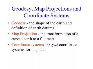
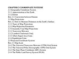
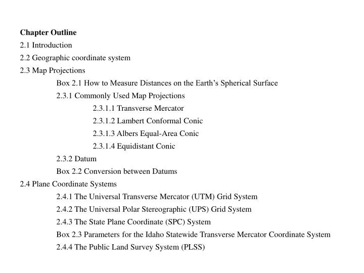
Chapter Outline 2.1 Introduction 2.2 Geographic coordinate system 2.3 Map Projections Box 2.1 How to Measure Distances on the Earth’s Spherical Surface 2.3.1 Commonly Used Map Projections 2.3.1.1 Transverse Mercator 2.3.1.2 Lambert Conformal Conic 2.3.1.3 Albers Equal-Area Conic

E N D
Chapter Outline 2.1 Introduction 2.2 Geographic coordinate system 2.3 Map Projections Box 2.1 How to Measure Distances on the Earth’s Spherical Surface 2.3.1 Commonly Used Map Projections 2.3.1.1 Transverse Mercator 2.3.1.2 Lambert Conformal Conic 2.3.1.3 Albers Equal-Area Conic 2.3.1.4 Equidistant Conic 2.3.2 Datum Box 2.2 Conversion between Datums 2.4 Plane Coordinate Systems 2.4.1 The Universal Transverse Mercator (UTM) Grid System 2.4.2 The Universal Polar Stereographic (UPS) Grid System 2.4.3 The State Plane Coordinate (SPC) System Box 2.3 Parameters for the Idaho Statewide Transverse Mercator Coordinate System 2.4.4 The Public Land Survey System (PLSS)
2.5 Working with Coordinate Systems in GIS Box 2.4 Coordinate Systems in ArcGIS
Applications: Map Projections and Coordinate Systems Task 1: Project a Shapefile from the Geographic Grid to a Plane Coordinate System Task 2: Import a Coordinate System Task 3: Project a Shapefile by Using a Predefined Coordinate System Task 4: Convert from one Coordinate System to Another
The top map shows two road coverages of Idaho and Montana based on different coordinate systems. The bottom map shows the road coverages based on the same coordinate system.
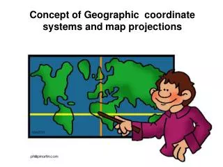
900N 600N, 1200W 300N, 600W Equator The geographic coordinate system
Secant Case Simple Case Conic Use of a geometric object to construct a map projection Cylindrical Azimuthal
Projection surface a c b Earth’s surface Scale factor a = 1.0000 b = 0.9996 c = 1.0000 The central meridian in this secant case transverse Mercator projection has a scale factor of 0.9996. The two standard lines on either side of the central meridian have a scale factor of 1.
(-,+) (+,+) (+,-) (-,-) The central parallel and the central meridian divides a map projection into four quadrants. Points within the NE quadrant have positive x- and y-coordinates, points within the NW quadrant have negative x-coordinates and positive y-coordinates, points within the SE quadrant have positive x-coordinates and negative y-coordinates, and points within the SW quadrant have negative x- and y-coordinates.
The Mercator and transverse Mercator projection of the United States. The central meridian is 90°W, and the latitude of true scale is the equator.
The Lambert conformal conic projection of the conterminous United States. The central meridian is 96°W, the two standard parallels are 33°N and 45°N, and the latitude of projection’s origin is 39°N.
North Pole b Equator a South Pole The semi-major axis is represented by a and the semi-minor axis is represented by b.
Magnitude of the horizontal shift from NAD27 to NAD83 in meters. See text for the definition of the horizontal shift. (By permission of the National Geodetic Survey.)
A UTM zone represents a secant-case transverse Mercator projection. CM is the central meridian, and AB and DE are the standard meridians. The standard meridians are placed 180 kilometers west and east of the central meridian. Each UTM zone covers 60 of longitude and extends from 840N to 800S. The size and shape of the UTM zone are exaggerated for illustration purposes.
State Plane Coordinate Systems for Washington, Oregon, and Idaho. The Lambert conformal conic projection is the basis for the Washington and Oregon coordinate systems, whereas the transverse Mercator projection is the basis for the Idaho coordinate system. The thinner lines are county boundaries.
R1E R1W R2E R2W 6 6 5 4 3 2 1 T2N 7 8 9 10 11 12 T1N 16 18 17 15 14 13 Base Line T1S R2E T1S 21 22 20 24 19 23 30 25 29 28 27 26 T2S 31 32 33 35 34 36 Boise Meridian An example of the Public Land Survey System (PLSS). The shaded survey township has the designation of T1S, R2E. T1S means that the survey township is south of the base line by one unit. R2E means that the survey township is east of the Boise (principal) meridian by 2 units. Each survey township is divided into 36 sections. Each section measures 1 mile-by-1 mile and has a numeric designation.
Conversion between datums, National Geodetic Survey http://www.ngs.noaa.gov/TOOLS/Nadcon/Nadcon.html Conversion between datums, U.S. Army Corps of Engineers http://crunch.tec.army.mil/software/corpscon/corpscon.html Geographic Coordinate Data Base (GCDB), Bureau of Land Management http://www.blm.gov/gcdb/