Download
1 / 11
170 likes | 577 Vues
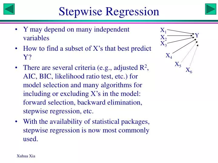
Stepwise Regression. Y may depend on many independent variables How to find a subset of X’s that best predict Y?

E N D
Stepwise Regression • Y may depend on many independent variables • How to find a subset of X’s that best predict Y? • There are several criteria (e.g., adjusted R2, AIC, BIC, likelihood ratio test, etc.) for model selection and many algorithms for including or excluding X’s in the model: forward selection, backward elimination, stepwise regression, etc. • With the availability of statistical packages, stepwise regression is now most commonly used. X1 Y X2 X3 X4 X5 X6
A Data Set for Multiple Regression Measurements on men involved in a physical fitness course at N. C. State University. Fitness is typically measured by oxygen intake rate (oxy) which is difficult (at least cumbersome when one is exercising oneself) to measure. The study goal is to develop an equation to predict oxy based on exercise tests rather than on oxygen consumption measurements. The dataset has 31 observations. The variables in the data set are: age (in years) weight (in kg) oxy (oxygen intake rate, ml per kg body weight per minute) runtime (time to run 1.5 miles, in minutes) rstpulse (heart rate while resting) runpulse (heart rate while running, at the same time when oxygen rate was measured) maxpulse (maximum heart rate recorded while running).
R Functions library(Hmisc) cor(myD,method="pearson|spearman") pairs(~age+weight+runtime+rstpulse+runpulse+maxpulse+oxy) rmat<-rcorr(as.matrix(myD), type="pearson|spearman") rmat print(rmat[1],digits=5) fit<-lm(oxy~age+weight+runtime+rstpulse+runpulse+maxpulse) anova(fit) summary(fit) full.model<-lm(oxy~age+weight+runtime+rstpulse+runpulse+maxpulse) best.model<-step(full.model,direction="backward") min.model<-lm(oxy~1) best.model<-step(min.model,direction="forward", scope="~age+weight+runtime+rstpulse+runpulse+maxpulse") new<-data.frame(specify values here) predict(fit,new,interval="confidence") predict(fit,new,interval="prediction")
Correlation matrix age weight oxy runtime rstpulse runpulse maxpulse age 1.00000 -0.23354 -0.30459 0.18875 -0.16410 -0.33787 -0.43292 0.2061 0.0957 0.3092 0.3777 0.0630 0.0150 weight -0.23354 1.00000 -0.16275 0.14351 0.04397 0.18152 0.24938 0.2061 0.3817 0.4412 0.8143 0.3284 0.1761 oxy -0.30459 -0.16275 1.00000 -0.86219 -0.39936 -0.39797 -0.23674 0.0957 0.3817 <.0001 0.0260 0.0266 0.1997 runtime 0.18875 0.14351 -0.86219 1.00000 0.45038 0.31365 0.22610 0.3092 0.4412 <.0001 0.0110 0.0858 0.2213 rstpulse -0.16410 0.04397 -0.39936 0.45038 1.00000 0.35246 0.30512 0.3777 0.8143 0.0260 0.0110 0.0518 0.0951 runpulse -0.33787 0.18152 -0.39797 0.31365 0.35246 1.00000 0.92975 0.0630 0.3284 0.0266 0.0858 0.0518 <.0001 maxpulse -0.43292 0.24938 -0.23674 0.22610 0.30512 0.92975 1.00000 0.0150 0.1761 0.1997 0.2213 0.0951 <.0001
rcorr in Hmisc oxy age weight runtime rstpulse runpulse maxpulse oxy 1.00 -0.30 -0.16 -0.86 -0.40 -0.40 -0.24 age -0.30 1.00 -0.23 0.19 -0.16 -0.34 -0.43 weight -0.16 -0.23 1.00 0.14 0.04 0.18 0.25 runtime -0.86 0.19 0.14 1.00 0.45 0.31 0.23 rstpulse -0.40 -0.16 0.04 0.45 1.00 0.35 0.31 runpulse -0.40 -0.34 0.18 0.31 0.35 1.00 0.93 maxpulse -0.24 -0.43 0.25 0.23 0.31 0.93 1.00 P oxy age weight runtime rstpulse runpulse maxpulse oxy 0.0957 0.3817 0.0000 0.0260 0.0266 0.1997 age 0.0957 0.2061 0.3092 0.3777 0.0630 0.0150 weight 0.3817 0.2061 0.4412 0.8143 0.3284 0.1761 runtime 0.0000 0.3092 0.4412 0.0110 0.0858 0.2213 rstpulse 0.0260 0.3777 0.8143 0.0110 0.0518 0.0951 runpulse 0.0266 0.0630 0.3284 0.0858 0.0518 0.0000 maxpulse 0.1997 0.0150 0.1761 0.2213 0.0951 0.0000 > print(rmat) oxy age weight runtime rstpulse runpulse maxpulse oxy 1.00 -0.30 -0.16 -0.86 -0.40 -0.40 -0.24 age -0.30 1.00 -0.23 0.19 -0.16 -0.34 -0.43 weight -0.16 -0.23 1.00 0.14 0.04 0.18 0.25 runtime -0.86 0.19 0.14 1.00 0.45 0.31 0.23 rstpulse -0.40 -0.16 0.04 0.45 1.00 0.35 0.31 runpulse -0.40 -0.34 0.18 0.31 0.35 1.00 0.93 maxpulse -0.24 -0.43 0.25 0.23 0.31 0.93 1.00
Backward elimination Start: AIC=58.16 oxy ~ age + weight + runtime + rstpulse + runpulse + maxpulse Df Sum of Sq RSS AIC - rstpulse 1 0.571 129.41 56.299 <none> 128.84 58.162 - weight 1 9.911 138.75 58.459 - maxpulse 1 26.491 155.33 61.958 - age 1 27.746 156.58 62.208 - runpulse 1 51.058 179.90 66.510 - runtime 1 250.822 379.66 89.664 Step: AIC=56.3 oxy ~ age + weight + runtime + runpulse + maxpulse Df Sum of Sq RSS AIC <none> 129.41 56.299 - weight 1 9.52 138.93 56.499 - maxpulse 1 26.83 156.23 60.139 - age 1 27.37 156.78 60.247 - runpulse 1 52.60 182.00 64.871 - runtime 1 320.36 449.77 92.917 the current model, i.e., without eliminating rstpulse
Forward addition Start: AIC=104.7 oxy ~ 1 Df Sum of Sq RSS AIC + runtime 1 632.90 218.48 64.534 + rstpulse 1 135.78 715.60 101.313 + runpulse 1 134.84 716.54 101.354 + age 1 78.99 772.39 103.681 <none> 851.38 104.699 + maxpulse 1 47.72 803.67 104.911 + weight 1 22.55 828.83 105.867 Step: AIC=64.53 oxy ~ runtime Df Sum of Sq RSS AIC + age 1 17.7656 200.72 63.905 + runpulse 1 15.3621 203.12 64.274 <none> 218.48 64.534 + maxpulse 1 1.5674 216.91 66.311 + weight 1 1.3236 217.16 66.346 + rstpulse 1 0.1301 218.35 66.516 Step: AIC=63.9 oxy ~ runtime + age Df Sum of Sq RSS AIC + runpulse 1 39.885 160.83 59.037 + maxpulse 1 14.885 185.83 63.516 <none> 200.72 63.905 + weight 1 5.605 195.11 65.027 + rstpulse 1 2.641 198.07 65.494 Step: AIC=59.04 oxy ~ runtime + age + runpulse Df Sum of Sq RSS AIC + maxpulse 1 21.9007 138.93 56.499 <none> 160.83 59.037 + weight 1 4.5958 156.24 60.139 + rstpulse 1 0.4901 160.34 60.943 Step: AIC=56.5 oxy ~ runtime + age + runpulse + maxpulse IVs whose addition will improve fit IVs whose addition will make it worse
Package leaps x<-as.matrix(myD) DV<-x[,1] IV<-x[,2:7] library(leaps) leaps(IV, DV, names=names(myD)[2:7], method="Cp") leaps(IV, DV, names=names(myD)[2:7], method=“adjr2")
Criteria used in model selection • Ra2 • Cp • SBC (BIC) • AIC • Significance level Burnham, K. P. and D. R. Anderson. 2002 Model selection and multimodel inference: a practical information-theoretic approach. 2nd ed. Springer. (Best book on model selection)