Download
1 / 61
611 likes | 751 Vues
Presented at IEEE GRSS Boston Section Meeting August 24, 2005 Choongyeun (Chuck) Cho. Anomaly Compensation and Cloud Clearing of AIRS Hyperspectral Data. Overview I. Problem statement Definition of anomaly Background

E N D
Presented at IEEE GRSS Boston SectionMeeting August 24, 2005 Choongyeun (Chuck) Cho Anomaly Compensation and Cloud Clearing of AIRS Hyperspectral Data
Overview I • Problem statement • Definition of anomaly • Background • Atmospheric InfraRed Sounder (AIRS), Advanced Microwave Souding Unit (AMSU), and Humidity Sounder for Brazil (HSB) instruments • Signal characterization and reduction of artifacts • Principal component analysis (PCA) and its variants • Artifacts in AIRS data
Overview II • Stochastic cloud-clearing • Background and prior work • Description of stochastic-clearing (SC) algorithm • Validation of stochastic-clearing algorithm • ECMWF • Physical clearing • Conclusion • Summary / contributions • Future work
Where Are We? • Problem statement • Definition of anomaly • Background • Signal characterization and reduction of artifacts • Stochastic cloud-clearing • Validation of SC algorithm • Conclusion
Problem Statement • What is hyperspectral data? • Hundreds or thousands of contiguous channels • What is anomaly? • Defined as an unwanted spatial or spectral signature, statistically distinct from its surrounding: • Given X and a priori information about Δ, what is best estimate of Δ or X? • A priori info about anomaly can have different forms: • Spectral statistical description, or usually ensembles • Spatial structure or texture • Joint spatial/spectral description ˜
Examples of Anomalies • Anomalies of AIRS data discussed in this talk • Instrumental noise • Noisy channels • AIRS data exhibits consistently noisy channels • Scan-line miscalibration • Resulting in striping patterns • Cloud contamination • Clouds generally make IR observations colder • Compensation for cloud impact is critical for accurate retrieval
Where Are We? • Problem statement • Background • AIRS/AMSU/HSB instruments • Signal characterization and reduction of artifacts • Stochastic cloud-clearing • Validation of SC algorithm • Conclusion
AIRS/AMSU/HSB Instruments on Aqua AIRS/HSB • Atmospheric InfraRed Sounder (AIRS) • 2378-channel infrared spectrometer covering 3.7-15.4μm • 1.1˚ FOV (13.5km at nadir) • Advanced Microwave Sounding Unit (AMSU) • 15 microwave channels • 3.3˚ FOV (40.5km at nadir) • Humidity Sounder for Brazil (HSB) • 1.1˚ FOV (13.5km at nadir, same as AIRS) • 4 microwave channels (150,190 GHz) • Scan motor failure since Feb 2003 AMSU “golfball”
Sample AIRS Brightness Temperatures AIRS sample spectra for 3-by-3 FOVs AIRS sample image Data: August 21, 2003 near Great Lakes
Where Are We? • Problem statement • Background • Signal characterization and reduction of artifacts • Principal component analysis (PCA) and its variants • Artifacts in AIRS data • Stochastic cloud-clearing • Validation of SC algorithm • Conclusion
Principal Component Analysis • Useful to characterize multivariate signal, and reduce dimensionality • Can be defined recursively (x: m-dim multivariate signal): • Solution: y = WTx where W = [w1|w2|…|wn], wi are eigenvectors of CXX which is often estimated • To reduce dimension, n << m • The resulting reconstructed signal: (PC filter)
Noise-Adjusted Principal Component • Principal components are sensitive to arbitrary scaling • Noise-adjusted PC (NAPC) • Normalize data before applying PCA: • Guarantees maximum SNR • What if noise variances are not known? • Need to be estimated using blind signal separation (BSS) technique such as Iterative Order and Noise (ION) estimation
Noise-Adjusted Principal Component • Typical “variances versus PC index” plot (truncated at 400) • NAPC shows sharper break than PC • 6 NAPCs explain 99.8% of variances Cumulative explained variance Scree plot for AIRS data Variance
Artifacts in AIRS Data • Measurements from a sensor can have different sources of artifacts • AIRS data has different types of unwanted artifacts • Instrumental noise • Noisy channels • Scan-line miscalibration • Each dot in the image is:
Instrumental Noise • Instrumental white noise is unavoidable • NAPC filtering provides adaptive noise filtering • NAPC filtering is extensively used in our stochastic clearing algorithm and noisy channel detector. Before After Histogram of difference
Noisy Channels I • Some channels are consistently noisy • These channels need to be excluded for further analysis and retrieval of physical parameters • Noisy channel detection is done with NAPC filtering such that a channel having 5σ even once is flagged “noisy” Block diagram of noisy channel detector
Noisy Channels II • AIRS science team has their own list of bad channels. • Detection rates for noisy and popping channels:
Scan-line Artifacts I • Miscalibrated scan-line results in stripes • A simple low-pass filter (in along-track direction) in NAPC domain corrects this artifact efficiently Block diagram of removing-stripe algorithm
Scan-line Artifacts II Original Images Processed Images • Results
Where Are We? • Problem statement • Background • Signal characterization and reduction of artifacts • Stochastic cloud-clearing • Background and prior work • Description of stochastic-clearing (SC) algorithm • Validation of SC algorithm • Conclusion
Background and Prior Work • What is cloud-clearing? • Cloudy radiances (or TB) cause inaccurate retrieval • Cloud-cleared radiances: radiances which would have been observed if FOV contains no clouds • Prior work on cloud-clearing • Ignore cloudy FOVs: only ~5% of AIRS FOVs are clear! • Physical cloud-clearing: iterate between estimation of physical parameters and calculation of observed radiance • Adjacent-pair clearing: use adjacent FOVs which have different fractional cloud cover • Purely spatial processing: restore 2-D temperature field from sparse clear data
Stochastic Clearing (SC) • How does stochastic clearing (SC) work? • SC estimates cloud contaminations solely based on statistics without using any physical models • Hyperspectral measurements may contain sufficient information about clouds in an obscured manner • Robust and stable training is necessary • Nonlinearity is accommodated using stratification (sea/land, latitude, day/night), multiplicative scan angle correction, etc. • Advantages of SC approach • Simple: SC does not require physical models (retrieval or radiative transfer). • Fast: Based on matrix addition and multiplication
Block Diagram of SC Algorithm D-cloud 2 TB’s 1 PC 1 Linear Operator A Linear Operator B 1 PC N Select/average FOV’s 3x3AIRS TB’s Less cloudy Cloudy Test 7 5 microwave l’s Land fraction Secant q More cloudy Linear Operator D Linear Operator C Cleared AIRS TB’s N N = 314 channels
Operators for SC Algorithm ECMWF + SARTA (v1.05)clear TB’s Trained with >1000 golfballs N AIRS TB’s Trained with >1000 golfballs Select & avg FOV’s N Operator A Operator B Find warmest † among 9 pixels* Noise-Adjusted PC’s 7 Operators C, D E S T I M A T O R L I N E A R + 3 Noise- Adjusted PC’s N Find coldestamong 9 pixels* AIRS D-cloud PC’s - TB AMSU ch. 5,6,8,9,10 5 * Warmest/coldest based on 11 4-mm channels peaking 1-3 km †Average 4 warmest pixels for 5-10 km WF, 9 for WF >10 km + 4 N + PC-1 TB’s secant q N Land fraction AIRS Cleared TB’s
Clearing Corrections vs ECMWF D’s 10 5 0 -5 -10 Red circles are best 37 percent “good golfballs” for nighttime ocean, all angles (operator C) Blue circles are cloudy golfballs (operator D) Classification Algorithm: “good golfballs” are below both 1K and 2K thresholds at operator B AIRS cleared – ECMWF/SARTA (oK) 1oK threshold -10 0 10 20 30 40 50 60oK Weighting function peak ~0.47 km, 2217.4 cm-1 10 5 0 -5 -10 2oK threshold Weighting function peak ~2.7 km, 2231.5 cm-1 -10 0 10 20 30 40 50 60 70oK
AIRS-ECMWF for 827 Channels 0 1 2 3 4 5 7 9 19 29 39 Best 22 percent of golfballs (operator C) Thresholds were 0.8K and 3K Nighttime ocean, all scan angles Includes all 4- and 15-mm channels plus one-fifth of the rest 314 good channels 314 good channels Weighting function peak height (km)
Where Are We? • Problem statement • Background • Signal characterization and reduction of artifacts • Stochastic cloud-clearing • Validation of SC algorithm • ECMWF • Physical clearing • Conclusion
ECMWF Data Set Used • ECMWF profiles are used to simulate cloud-cleared TB’s via SARTA v1.05 radiative transfer, for all scan angles, 314 channels • Global, 3 days: 8/21, 9/3, 10/12/03 (L1B v3.0.8) • AIRS instrument noise reduced by averaging 1, 4, or 9 of the warmest* 15-km pixels for weighting function peaks 0-5, 5-10, and >10 km, respectively • Used 1000 golf balls to regress each of 10 categories based on day/night, land/sea, and |lat|<40 or 40<|lat|<70
RMS Difference (AIRS-ECMWF) for Ocean • For best 28%: sea + |lat|<40º + day (best for sea)
RMS Difference (AIRS-ECMWF) for Land • For best 28%: land + |lat|<40º + night (best for land)
Cloud-cleared AIRS vs. ECMWF (best 28%) • RMS difference (oK) between cloud-cleared AIRS and ECMWF/SARTA, 10 different estimators • RMS > 0.7 K are boxed • Excellent agreement for ocean and equatorial regions • Degradation over daytime land near surface 0.38 0.4 0.86 0.91 1.68 0.77 1.36 1.48 0.78 1.19 0.27 0.29 0.54 0.57 0.94 0.38 0.75 0.84 0.44 0.70 0.28 0.30 0.45 0.45 0.34 0.29 0.33 0.41 0.33 0.39 0.23 0.27 0.34 0.36 0.25 0.24 0.28 0.34 0.26 0.31 0.24 0.27 0.33 0.35 0.23 0.25 0.26 0.24 0.28 0.27
Global Cloud-Clearing Images (2392.1cm-1) • SC applied to 8/21/2003 descending orbits (L1B v4.0.9) • 2392.1cm-1, WF peak=0.23 km Observed AIRS Cloud-cleared (best ~78%)
Global Cloud-Clearing Images (2392.1cm-1) Observed AIRS CC residual • CC Residual = Spatially high-pass filtered version of CC • WF peaks at 0.23 km
Cloud-Clearing Images and Sea Surf. Temperature Observed Cleared SST AIRS 2390.1cm-1: near Hawaii • Angle-corrected TB images at window channels • Clearing works well even if there is no hole (clear FOV) AIRS 2399.9cm-1: near SW Indian Ocean
Validation with Physical Clearing Visible vs. AIRS 8.15-m Data 140 5 5 290 120 285 100 15 15 280 80 275 25 25 60 270 40 35 35 265 20 260 45 45 Visible Ch 3 1227.7 cm-1 270 265 260 255 250 Granule 91(9/6/02) (solar reflection) Channel 1284(H2O)
Determination of AIRS Cloud-Cleared Brightness Temperature Baselines Stochastic CC Clear Mask † Fitted ‡ Channel 1284 (H2O) (1227.7 cm-1) Granule 91 (9/6/02) Indian Ocean, LAT -26.3, LON 70.2 † Clear mask determined from Visible Ch 3, Brown being clear ‡ Polynomial fit: 4th order in scan angle, 3rd order downtrack
Stochastic versus Physical Cloud-Cleared8.15-m Brightness Temperatures Stochastic Clearing -Visible Ch 3 Physical Clearing Channel 1284 (H2O) (1227.7 cm-1) Granule 91 (9/6/02) Indian Ocean, LAT -26.3, LON 70.2 Filter subtracts cloud-cleared baseline and convolves with 33 boxcar
Correlation Coefficients: Visible (v3) vs. Cloud-Cleared 8.15-m AIRS TB’s AIRS channel 1284(1227.7 cm-1)(water vapor)September 6, 2002 Lon -26.3/Lat 70.2 Indian Ocean Lon -12.5/Lat -106.1 Eastern Southern Pacific
Stochastic and Physics-BasedCloud-Cleared Window Channel TB Stochastic Clearing Physics-Based Clearing* Channel 2121 (2399 cm-1), WF peak ~200m 9/6/02 North of Bermuda * Note that the physical clearing is most recent version (PGE v4.0.0), calculated this week.
Where Are We? • Problem statement • Background • Signal characterization and reduction of artifacts • Stochastic cloud-clearing • Validation of SC algorithm • Conclusion • Summary / contributions • Future work
Summary • Anomaly compensation techniques are discussed based on signal processing techniques (NAPC and ION) and nonlinear estimators • Anomalies: Gaussian instrument noise, noisy channels, scan-line miscalibration, and cloud contamination • Stochastic clearing (SC) algorithm tested to be successful using different validation schemes: • ECMWF • Sea surface temperature (SST) • Physical algorithm
Contributions: Methodology • We developed “architected nonlinear estimators”, taking advantage of simplicity of linear estimator and robustness of general nonlinear estimator • NAPCs are used to reduce dimension and suppress noise, making more robust and stable estimation • Prior knowledge (either spectral or spatial) about anomaly is utilized to meaningfully structure a nonlinear estimator Architected Nonlinear Estimator General Nonlinear Estimator Linear Estimator Prior info about anomaly Dimension reduction • May be unstable • Complex/Slow • Most powerful • Stable • Simple/Fast • Less powerful • Stable • Simple/Fast • Sufficiently powerful
Contributions: Stochastic Clearing • SC algorithm developed based on anomaly compensation and nonlinear estimation techniques: • Enjoys excellent agreement with numerical weather prediction model (ECMWF) • Performs superior to physical clearing • Very fast: depends on matrix addition and multiplication; consists of 664 lines of Matlab code, ~20 minutes to cloud clear an entire day of AIRS data on ordinary PC • Clearing at extreme scan angles is good; hole-hunting using high spatial resolution may not be essential for cloud-clearing
Future Work • Anomaly compensation theory • Optimization of combining spectral and spatial processing • More extensive spectral processing techniques • SC algorithm • Joint cloud-clearing and retrieval • Better model for nonlinearities • Optimum architecture for SC algorithm using efficient design-of-experiment approach
Where Are We? • Problem statement • Background • Signal characterization and reduction of artifacts • Stochastic cloud-clearing • Validation of SC algorithm • Conclusion That’s all, folks. Any questions?
Global Cloud-Clearing Images (2392.1cm-1) CC residual AIRS CC • Zoom-in images in Southeastern Pacific • WF peaks at 0.23 km
Determination of AIRS Cloud-Cleared Brightness Temperature Baselines Stochastic CC Cloud Mask † Fitted ‡ Channel 1284 (H2O) (1227.7 cm-1) Granule 91 (9/6/02) Indian Ocean, LAT -26.3, LON 70.2 † Brown being clear (accepted) ‡ Polynomial fit: 4th order in scan angle, 3rd order downtrack
SC Validation w.r.t. SST • NCEP sea surface temperature
AIRS Stratified Stochastic Cloud Clearing First-pass results Multiplicative Scan-angle Stratified results 46% golfballs good 54% rejected 0.8K threshold (AIRS cleared radiance) – (ECMWF/SARTA) (oK) 46% golfballs good 54% rejected 3K threshold Estimate of cloud-clearing radiance correction (oK)