Download
1 / 2
20 likes | 166 Vues
Consider temporal variation in growth rates. GOOD = 1.7. P GOOD = 0.5. P BAD = 0.5. BAD = 0.4. (1) Calculate the long-term growth rate ( ) for 1,2,3,4 and 5 sub-populations Plot versus # sub-populations. What is the minimum # sub-populations for this to be a source? .

E N D
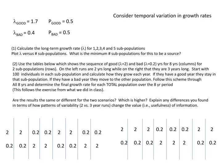
Consider temporal variation in growth rates GOOD = 1.7 PGOOD = 0.5 PBAD = 0.5 BAD = 0.4 (1) Calculate the long-term growth rate () for 1,2,3,4 and 5 sub-populations Plot versus # sub-populations. What is the minimum # sub-populations for this to be a source? (2) Use the tables below which shows the sequence of good (=2) and bad (=0.2) yrs for 8 yrs (columns) for 2 sub-populations (rows). On the left runs are 2 yrs long while on the right that they are 3 years long. Start with 100 individuals in each sub-population and calculate how they grow each year. If they have a good year they stay in that sub-population. If they have a bad year they move to the other population. Follow this scheme through All 8 yrs and determine the final growth rate for each TOTAL population over the 8 yr period (This follows the exercise from what we did in class). Are the results the same or different for the two scenarios? Which is higher? Explain any differences you found in terms of how patterns of variability (2 vs. 3 year runs) change the value (i.e., usefulness) of information. 2 2 0.2 0.2 0.2 2 2 0.2 0.2 0.2 2 2 2 0.2 0.2 2 0.2 0.2 2 2 0.2 0.2 0.2 0.2 2 2 0.2 0.2 2 2
Hotspot Original Area (km2) % Protected Birds spp mammal spp Tropical Andes 1,258,000 6.3 1,666 414 Mesoamerica 1,155,00012.0 1193 521 *Wallacea347,0005.9 697201 Madagascar 594,000 1.9 359112 *Philippines301,000 1.3566201 *Polynesia46,00010.725416 Indo-Burma 2,060,0007.81170329 (2) Plot log spp (bird and mammals separately) versus log area (on graph paper or in excel!) Is it what you would predict? If not explain why not. Use the table above to calculate the number of species that will remain if all the area is taken away for wildlife except what is currently protected. Calculate in two steps: first, loss of endemics and second, relaxation to an island state (note the hotspots with a (*) are already islands, so only calculate the first decline – Madagascar and Indo-Burma are also islands, but very large ones so they can become new island states) To do this use the relationship: # Species = a(Area)C where ‘a’ and ‘c’ are constants. For ‘a’, you use the present number of species for each site (e.g., for birds in Tropical Andes a=1,666). For ‘c’ use the appropriate values from lecture (c varies for the two types of losses). For Area, you will use the proportion that remains (e.g., Tropical Andes Area=0.063). Last, read some background on the 7 different areas and indicate likely species of birds and mammals (I mean real species – so a little research is necessary) will disappear from each hotspot – explain your answer.