Download
1 / 12
140 likes | 305 Vues
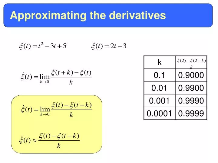
Approximating the derivatives. Numerical ODE (1D). Initial Value Problem:. Example:. Approximate . Numerical ODE (1D). Example:. Approximate . Forward Euler Method. Forward Euler Method. Example:. Numerical ODE (1D). Example:. function [xi,ti]=feuler(t0,T,n,xi_0) k=(T-t0)/n;

E N D
Numerical ODE (1D) Initial Value Problem: Example: Approximate
Numerical ODE (1D) Example: Approximate
Forward Euler Method Forward Euler Method Example:
Numerical ODE (1D) Example: function [xi,ti]=feuler(t0,T,n,xi_0) k=(T-t0)/n; ti=[t0:k:T]; F=inline('xi+4*exp(0.5*t)+5','xi','t'); xi(1) = xi_0; for i=2:n+1 xi(i) = xi(i-1)+k*F(xi(i-1),ti(i-1)); end [xi,ti]=feuler(0,1,100,-5) plot(ti,xi,'bo-')
Crank–Nicolson Method Forward Euler Method Backward Euler Method Crank-Nicolson Method Larson Book Each of these three method have its own characteristics regarding accuracy, stability, and computational cost. Loosely speaking, forward Euler is very fast, backward Euler numerically stable, and Crank-Nicolson the most accurate.
Numerical ODE (System) System of ODEs: Numerical: M nxn matrix Forward Euler Method Crank-Nicolson Method
Numerical ODE (System) Special Case: M nxn matrix A nxn matrix Crank-Nicolson Method
Numerical ODE (System) Example: function [xi,t]=cnm(t0,T,n,xi_0) k=(T-t0)/n; t=[t0:k:T]; b=inline('[t.^2-1;3.*t+2]'); A=[1,0;0,1]; M=[2,1;1,2]; MpA=M+(k/2)*A; MmA=M-(k/2)*A; xi(:,1) = xi_0; for i=2:n+1 bb= (k/2)*( b(t(i)) + b(t(i-1)) ); rhs = MmA*xi(:,i-1)+bb; xi(:,i) = MpA\rhs; end with the initial condition Use Crank-Nicolson Method to solve the system. Then plot the two components of the solution.
Numerical ODE (System) Exercise: with the initial condition Use Crank-Nicolson Method to solve the system. Then plot the two components of the solution.
Numerical ODE (2ed order) 2ed order: Introduce a new varible to reduce it into 1st order
Numerical ODE (System) Example: with the initial condition Use Crank-Nicolson Method to solve the system. Then plot the two components of the solution.