Lecture 9. MIPS Processor Design – Single-Cycle Processor Design

1. 2010 R&E Computer System Education & Research Lecture 9. MIPS Processor Design – Single-Cycle Processor Design Prof. Taeweon Suh Computer Science Education Korea University

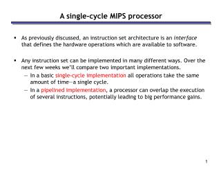
2. Single-Cycle MIPS Processor • Again, microarchitecture (CPU implementation) is divided into 2 interacting parts • Datapath • Control

3. Single-Cycle Processor Design • Let’s start with a memory access instruction - lw • Example: lw $2, 80($0) • STEP 1: Instruction Fetch

4. Single-Cycle Processor Design • STEP 2: Decoding • Read source operands from register file Example: lw $2, 80($0)

5. Single-Cycle Processor Design • STEP 2: Decoding • Sign-extend the immediate Example: lw $2, 80($0) module signext(input [15:0] a, output [31:0] y); assign y = {{16{a[15]}}, a}; endmodule

6. Single-Cycle Processor Design • STEP 3: Execution • Compute the memory address Example: lw $2, 80($0)

7. Single-Cycle Processor Design • STEP 4: Execution • Read data from memory and write it back to register file Example: lw $2, 80($0)

8. Single-Cycle Processor Design • We are done with lw • CPU starts fetching the next instruction from PC+4 module adder(input [31:0] a, b, output [31:0] y); assign y = a + b; endmodule adder pcadd1(pc, 32'b100, pcplus4);

9. Single-Cycle Processor Design • Let’s consider another memory access instruction - sw • swinstruction needs to write data to data memory Example: sw $2, 84($0)

10. Single-Cycle Processor Design • Let’s consider arithmetic and logical instructions - add, sub, and, or • Write ALUResult to register file • Note that R-type instructions write to rd field of instruction (instead of rt)

11. Single-Cycle Processor Design • Let’s consider a branch instruction - beq • Determine whether register values are equal • Calculate branch target address (BTA) from sign-extended immediate and PC+4 Example: beq $4,$0, around

12. Single-Cycle Datapath Example • We are done with the implementation of basic instructions • Let’s see how orinstruction works out in the implementation

13. Single-Cycle Processor - Control • As mentioned, CPU is designed with datapath and control • Now, let’s delve into the control part design

14. Control Unit Opcode and funct fields come from the fetched instruction

15. ALU Implementation and Control N = 32 in 32-bit processor adder slt: set less than Example: slt $t0, $t1, $t2 // $t0 = 1 if $t1 < $t2

16. Control Unit: ALU Control • Implementation is completely dependent on hardware designers • But, the designers should make sure the implementation is reasonable enough • Memory access instructions (lw, sw) need to use ALU to calculate memory target address (addition) • Branch instructions (beq, bne) need to use ALU for the equality check (subtraction)

17. Control Unit: Main Decoder 1 1 0 0 0 0 10 1 0 0 1 00 1 0 0 00 X 1 0 1 X 01 X 0 X 1 0 0

18. How about Other Instructions? • Hmmm.. Now, we are done with the control part design • Let’s examine if the design is able to execute other instructions • addi Example: addi $t0, $t1, -14

19. Control Unit: Main Decoder 0 0 1 00 0 1 0

20. How about Other Instructions? • Ok. So far, so good… • How about jump instructions? • j

21. How about Other Instructions? • We need to add some hardware to support the j instruction • A logic to compute the target address • Mux and control signal

22. Control Unit: Main Decoder • There is one more output in the main decoder to support the jump instructions • Jump

23. Verilog Code - Main Decoder and ALU Control module maindec(input [5:0] op, output memtoreg, memwrite, output branch, alusrc, output regdst, regwrite, output jump, output [1:0] aluop); reg [8:0] controls; assign {regwrite, regdst, alusrc, branch, memwrite, memtoreg, jump, aluop} = controls; always @(*) case(op) 6'b000000: controls <= 9'b110000010; // R-type 6'b100011: controls <= 9'b101001000; // lw 6'b101011: controls <= 9'b001010000; // sw 6'b000100: controls <= 9'b000100001; // beq 6'b001000: controls <= 9'b101000000; // addi 6'b000010: controls <= 9'b000000100; // j default: controls <= 9'bxxxxxxxxx; // ??? endcase endmodule module aludec(input [5:0] funct, input [1:0] aluop, output reg [2:0] alucontrol); always @(*) case(aluop) 2'b00: alucontrol <= 3'b010; // add 2'b01: alucontrol <= 3'b110; // sub default: case(funct) // RTYPE 6'b100000: alucontrol <= 3'b010; // ADD 6'b100010: alucontrol <= 3'b110; // SUB 6'b100100: alucontrol <= 3'b000; // AND 6'b100101: alucontrol <= 3'b001; // OR 6'b101010: alucontrol <= 3'b111; // SLT default: alucontrol <= 3'bxxx; // ??? endcase endcase endmodule

24. Verilog Code – ALU module alu(input [31:0] a, b, input [2:0] alucont, output reg [31:0] result, output zero); wire [31:0] b2, sum, slt; assign b2 = alucont[2] ? ~b:b; assign sum = a + b2 + alucont[2]; assign slt = sum[31]; always@(*) case(alucont[1:0]) 2'b00: result <= a & b2; 2'b01: result <= a | b2; 2'b10: result <= sum; 2'b11: result <= slt; endcase assign zero = (result == 32'b0); endmodule

25. Single-Cycle Processor Performance • How fast is the single-cycle processor? • Clock cycle time (frequency) is limited by the critical path • The critical path is the path that takes the longest time • What do you think the critical path is? • The path that lwinstruction goes through

26. Single-Cycle Processor Performance • Single-cycle critical path: Tc = tpcq_PC + tmem + max(tRFread, tsext) + tmux + tALU + tmem + tmux + tRFsetup • In most implementations, limiting paths are: memory (instruction and data), ALU, register file. Thus, Tc = tpcq_PC + 2tmem + tRFread + 2tmux + tALU + tRFsetup

27. Single-Cycle Processor Performance Example Tc = tpcq_PC + 2tmem + tRFread + 2tmux + tALU + tRFsetup = [30 + 2(250) + 150 + 2(25) + 200 + 20] ps = 950 ps fc = 1/Tc fc = 1/950ps = 1.052GHz • Assuming that the CPU executes 100 billion instructions to run your program, what is the execution time of the program on a single-cycle MIPS processor? Execution Time = (#instructions)(cycles/instruction)(seconds/cycle) = (100 × 109)(1)(950 × 10-12 s) = 95 seconds