Download
1 / 49
490 likes | 557 Vues
Several topics. Ocean studies (v5 reprocessed SSS). Version 6 versus version 5. -v602 in May 2011 (land/ice contamination; ARGO colocations) -v610 in December/descending (sun?). Ice coverage Rain-Roughness effect/ 2-step algo. -South Pacific Maximum Salinity

E N D
Several topics Ocean studies (v5 reprocessed SSS) Version 6 versus version 5 -v602 in May 2011 (land/ice contamination; ARGO colocations) -v610 in December/descending (sun?) Ice coverage Rain-Roughness effect/ 2-step algo -South Pacific Maximum Salinity -North Atlantic Maximum Salinity (SPURS) -Variability of SSS: effects of rain/roughness/interpolation smoothing
Version 6 versus version 5J. Boutin, N. Martin, X. Yin -L1v602 (land & ice contamination worse in L1v602 than in v5.5 not shown in this presentation); colocs with ARGO. -Sun impact on descending orbits in December with L1v610?
Mai 2011 – L1 v602 + L2 v6 versus v5 reprocessed Land and ice contamination worse in L1 v602!
Far from continents (>700km), comparisons with ARGO : colocs +/-9days, +/-50km ; 10 -25 Mai 2011 Mai 2011 – L1 v602 + L2 v6 versus v5 reprocessed
Far from continents, comparisons with ARGO : colocs +/-9days, +/-50km ; 10 -25 Mai 2011 Orbit A [45S;45N] : v5 : N= 1674 mean=-0.16 std=0.417 v6ref : N= 1674 mean=-0.13 std=0.396 v6a3tec : N= 1674 mean=-0.13 std=0.396 Orbit D [45S;45N] : v5 : N= 1605 mean= 0.04 std=0.448 v6ref : N= 1605 mean= 0.06 std=0.456 v6a3tec : N= 1605 mean=-0.05 std=0.398 Orbit A+D [45S;45N] : v5 : N= 1943 mean=-0.07 std=0.360 v6ref : N= 1943 mean=-0.05 std=0.346v6a3tec : N= 1943 mean=-0.10 std=0.321 Mai 2011 – L1 v602 + L2 v6 versus v5 reprocessed L1 v602 gives equal or very slightly improved performance wrt v5; L2 v6a3tec improves much more
Are descending orbits in the northern hemisphere in December less noisy in v610 than in v5 repr. ?X. Yin, J. Boutin Look at std(Tbsmos-Tbmodel) wrt radiometric accuracy over one descending orbit 20121217T032055_20121217T041408 between 5°N and 35°N Flags of border, sun point and suntails are applied. The gridpoints in the FOV with number of measurements less than 30 are forced to be blank.
(in v5, most retrieved SSS north of 5°N in Dec are flagged December/Descending! )
Std(Txsmos-Txmodel)/Radiometric accuracy V5 V6 V6 less noisy than v5 but still some remaining anomalous signatures
Std(Tysmos-Tymodel)/Radiometric accuracy V5 V6 V6 less noisy than v5 but still some remaining anomalous signatures
Std(Txsmos-Txmodel) V5 V6 V6 less noisy than v5 but still some remaining anomalous signatures
Std(Tysmos-Tymodel) V5 V6 V6 less noisy than v5 but still some remaining anomalous signatures
SMOS-ECMWF ice coverage wrt OSTIA ice coverage J. Boutin, N. Martin,C. Banks
Motivation • At the ESA LPS 2013 Chris Banks suggests that SMOS was biased close to ice as detected by OSTIA • In v5 (and v600), in L2OS processor threshold for ice concentration is not put to 0% but to 30% • =>look at difference between considering a threshold=0% or 30% • => look at difference between SMOS-ECMWF & OSTIA ice concentration
Data & Method • All tests are performed on 15 May 2011 • All SMOS-ECMWF ice concentrations along SMOS orbits on 15 May are averaged
Zoom on some regions of 0% & 30% threshold on SMOS/ECMWF ice concentration Ice concentration between 30% and 0% concerns often a band of ~1° in latitude or even larger; this is not negligible and from a physical point of view it is necessary to consider 0%!
SMOS SSS close to ECMWF-SMOS ice mask (purple 0%, black 30%) Probably due to other sortings, SMOS SSS is not retrieved very close to SMOS-ECMWF ice on 15 May asc orbits
SMOS SSS close to ECMWF-SMOS ice mask (purple 0%, black 30%) The southern limit of SMOS retrieval is closer to OSTIA than to ECMWF ice concentration =0%
Conclusion Study in progress; some strange across track biases close to ice (TBC) but it was v6!!! It would be safer to put threshold to 0% instead of 30% on percentage of ECMWF ice coverage (although it seems that other tests in L2OS already discard data within 0 and 30%)
Rain-Roughness effect : what two-step algorithm tells usX. Yin, J. Boutin, N. Martin
WSECMWF - WSSSMIS North Eq Pac East Eq Pac rWSOP - WSSSMIS rWStwostep - WSSSMIS In regions with large ECMWF-SSMI WS differences, 2-step retrieved SMOS WS closer to SSMI WS; 2-step method more sensitive to problems near continents and RFI regions
East Eq Pac region WSECMWF - WSSSMIS rWSOP - WSSSMIS rWStwostep - WSSSMIS In regions with large ECMWF-SSMI WS differences, 2-step retrieved SMOS WS closer to SSMI WS; 2-step method more sensitive to problems near continents and RFI regions
Statistics in August 2010 –Ascending orbits(EEP contains low WS that may create an additional problem)
SMOS SSS – ARGO SSS5°N-15°N Pacific Ocean SMOS SSS [1cm]– ARGO SSS [5m] correlated with SSM/I rain rates (within -80mn;+60mn from SMOS passes) Still strong correlation with RR when an alternative SMOS roughness correction scheme is used (poster Yin et al., 4P-117) Operational SSS Two step SSS Change in roughness by raindrop: a second order effect wrt vertical stratification (account for less than 20% of observed SSSsmos-SSSargo difference) Boutin et al., Ocean Science, 2013 Method described in 4P-117
Conclusions As suggested by 2-step algorithm, rain induced roughness is an order of magnitude smaller than rain-stratification effect 2-step algorithm very useful to detect peculiar roughness (not wel modelled with ECMWF WS) but very sensitive to land contamination, RFI...
Scientific studies that used v5 reprocessed SSS -South Pacific Maximum Salinity -North Atlantic Maximum Salinity (SPURS) -Variability of SSS: effects of rain/roughness/interpolation smoothing
In press Figure 1. (a) Mean 1990-2011 modelled mixed-layer salinity. The blue lines represent the Matisse Ship routes of 2010 and 2011 discussed in the main text. (b) Mean Evaporation – Precipitation (E-P) based on ERAi; units are mm/day. Overplotted as arrows are the mean modelled surface currents. The 0 isohyet is shown on both panels with a bold black solid line.
SMOS SSS, modelled SSS and ship SSS Over 8 VOS TSG transects (averaged over 20-30km): For a collocation radius of 9 days and 50 km, std difference : Between SMOS and in-situ SSS : 0.20 Between modelled and in-situ SSS : 0.26 (mean biases -0.08 and 0.07, respectively) Comparison between near-surface salinity data derived from (black line) the TSG instrument installed on board M/V Matisse and the collocated SSS: (dashed line) modelled and (dotted line) SMOS values. The Matisse salinity values were obtained during 20-27 February 2011 along the northern shipping line shown in Figure 1a. (Hasson et al, JGR, 2013 in press) Model: ORCA025.L75-MRD911 run by french Drakkar group
Salinity budget as derived from model analysis Evaporation-Precipitation (~0.7pss yr-1) balanced by the horizontal salinity advection (~--0.35 pss yr-1) and processes occurring at the mixed layer base (~-0.35 pss yr-1). Mean mixed-layer salinity budgets in the high-salinity regions bounded by the 35.6, 36 and 36.4 isohalines (Hasson et al, JGR, 2013 in press)
Seasonal and interannual displacement of 36 isohalines Very consistent seasonal variation of longitudinal displacement between SMOS and modelled SSS (according to ship SSS, max of modelled SSS could be too north) (a) Monthly and (b) annual mean positions of the modelled 36-isohaline. On both panels the colored dots and stars show respectively the barycentre of the modelled and SMOS-derived 36 isohalines (Hasson et al, JGR, 2013 in press) Model: ORCA025.L75-MRD911 run by french Drakkar group
SMOS-LOCEAN activities in SPURS region(Hernandez et al., Kolodziejczyk et al., 2013, in prep. JGR-SMOS-AQUARIUS)
Ship data from 07/2011 to 12/2012: 14 transects SMOS senses mesoscale variability (≠ ISAS)(Hernandez et al., Kolodziejczyk et al., 2013, in prep. JGR) SMOS vs TSG SSS anomaly (0.25° resol.) ISAS vs TSG SSS anomaly (0.25° resol.) ISAS –climato SSS SMOS –climato SSS Once monthly biases are corrected, SMOS senses variability with a RMSE= 0.14 TSG –climato SSS TSG –climato SSS
SMOS and in situ salinity: rain, roughness and interpolation effects J. Boutin1, N. Martin1, J.L. Vergely2, X. Yin1, G. Reverdin1, F. Gaillard3, O. Hernandez 1, N. Reul4 1 LOCEAN/CNRS, Paris, 2 ACRI-st, Paris, 3 LPO/IFREMER, Brest, 4 LOS/IFREMER, Toulon, France
Motivation: SMOS S1cm maps versus in situ S~5m maps SSS August 2010 Rain Rate (SSMI) ISAS ~5m depth ~3°smoothing SMOS 1cm depth 100x100km 2 averages ITCZ SPCZ CATDS-CEC/LOCEAN_v2013 product
Outline -Assessment of Levenberg and Marcquardt (LM) retrieved SSS error: SMOS SSS variability within 100km-1month in and out of rainy regions: comparison with SMOS SSS error predicted by LM. -Alternative roughness retrieval: the 2-step algorithm of X.Yin =>weak effect of rain-roughness on SMOS-ARGO SSS: first order is vertical stratification -Monthly SMOS SSS maps wrt in situ derived maps (ISAS): -differences linked to rain-stratification -differences linked to interpolation smoothing
Data & Methods SATELLITE SMOS SSS ESA v5 reprocessing SSS at 1cm depth ; ~40km resolution or averaged (CATDS-CEC/LOCEAN_v2013 product available at www.catds.fr) ; focus on August 2010 monthly maps Rain Rate: -SSM/I (RemSSS: www.ssmi.com)0.25° resolution; SMOS SSS colocated within -80mn, +40mn IN SITU SSS ARGO INDIVIDUAL PROFILES ‘SSS’ between 10m and 4m depth; Colocation with SMOS within +/-5days, +/-50km CORIOLIS GDAAC: http://www.coriolis.eu.org ARGO + TSG OPTIMAL INTERPOLATED SSS MAPS (ISAS) Monthly maps from In-Situ Analysis System v6 – Correlation scale ~300km http://wwz.ifremer.fr/lpo/SO-Argo/Products/Global-Ocean-T-S
Method for building SMOS SSS maps(CATDS LOCEAN_CEC_v2013) • Monthly SSS average over 100x100km2 • weighted by each SSSj resolution (Rj) and theoretical uncertainty on retrieved SSS (ej) derived by the L.M. algorithm ( depends on NTb, dTb/dSSS,...) • Mean theoretical error on single SMOS SSS is computed with same weights e e e eSSS ESSS =
SMOS SSS theoretical error & observed variability Mean theoretical error on single SMOS SSS (~43km resolution): eSSS Standard deviation of L2OS SMOS retrieved SSS over 1 month in 100x100km2: SSS (if no natural variability, no bias on SMOS SSS, errorSSS~SSS)
SMOS SSS theoretical error & variability:SSS - eSSS Large SSS close to the coast (large and variable SMOS SSS biases) 750km
SMOS SSS theoretical error & variability:SSS - eSSS Large SSS close to the coast (large and variable SMOS SSS biases) but also in tropical regions Influence of rain on SSS – eSSS ? Several possible causes: -natural variability (rain is an intermittent process) -rain-roughness artefact on SSS retrieval
SMOS SSS theoretical error & variability:Correlation with rain SSS – eSSS versus monthly SSMI Rain Rate SSS – eSSS ~0.6 * RR : -SSSvar2 ~ SSS2 - eSSS2 For RR=0.5mm/hr & eSSS=0.6 => SSS natural variability ~0.6 order of magnitude need to be further checked with in situ ground truths Tropical Pacific 5N-15N
SMOS SSS – ISAS SSS What is the impact of a correction for rain stratification effect as seen on SSSsmos-SSSargo? After masking areas close to continents and RFIS: SMOS SSS-ISAS SSS Global Ocean: moy=-0.16 (std=0.36) 30°S-30°N: moy=-0.18 (std=0.28)
SMOS S1cm – ARGO S~5m =fn(RR) Region close to SPCZ Region close to ITCZ Boutin et al. 2013 SMOS S~5m ~ SMOS S1cm + 0.19 RR
Effect of Rain correction on monthly SSS A small correction (not the same color scales!!) SSScorr-SSS SSScorr-SSSisas SSSsmos – SSSisas : Without rain correction: moy=-0.16 (std=0.36) moy=-0.18 (std=0.28) With rain correction: moy=-0.15 (std=0.36) moy=-0.17 (std=0.28) Global Ocean: 30°S-30°N: Vertical stratification of S linked to rain is not responsible for the main differences between SSSsmos-SSSisas – Influence of ISAS optimal interpolation (~300km)???
Effect of ISAS interpolation SSSsmos_like_ISAS - SSSisas SSSsmos- SSSisas moy=-0.16 (std=0.36) moy=-0.18 (std=0.28) Global: moy=-0.09 (std=0.22) 30°N-30°S: moy=-0.09 (std=0.21)
Summary -SMOS SSS theoretical error in very good agreement with the SMOS SSS observed variability within 100x100km2 and one month, except close to continents, RFIs and in rainy regions. -In rainy regions, salinity natural variability is expected to be large (temporally, spatially and vertically): -SMOS suggests S1cm variability due to time/space variability over one month ~0.6 for a monthly RR=0.5mm/hr. This order of magnitude should be checked in future studies with surface ground truth. -When averaged over one month, the rain induced vertical salinity difference between 5m & 1cm is small (<0.1). -When SMOS SSS interpolated similarly to in situ SSS : precision on monthly SMOS SSS smoothed at ~3° resolution ~0.2 between 30°N-30°S. -