Download
1 / 39
550 likes | 1.66k Vues
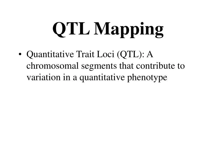
QTL Mapping. Quantitative Trait Loci (QTL): A chromosomal segments that contribute to variation in a quantitative phenotype. Maize Teosinte tb-1 / tb-1 mutant maize. Mapping Quantitative Trait Loci (QTL) in the F2 hybrids between maize and teosinte.

E N D
QTL Mapping • Quantitative Trait Loci (QTL): A chromosomal segments that contribute to variation in a quantitative phenotype
Maize Teosinte tb-1/tb-1 mutant maize
Mapping Quantitative Trait Loci (QTL) in the F2 hybrids between maize and teosinte
Nature432, 630 - 635 (02 December 2004)The role of barren stalk1 in the architecture of maize ANDREA GALLAVOTTI(1,2), QIONG ZHAO(3), JUNKO KYOZUKA(4), ROBERT B. MEELEY(5), MATTHEW K. RITTER1,*, JOHN F. DOEBLEY(3), M. ENRICO PÈ(2) & ROBERT J. SCHMIDT(1) 1 Section of Cell and Developmental Biology, University of California, San Diego, La Jolla, California 92093-0116, USA2 Dipartimento di Scienze Biomolecolari e Biotecnologie, Università degli Studi di Milano, 20133 Milan, Italy3 Laboratory of Genetics, University of Wisconsin, Madison, Wisconsin 53706, USA4 Graduate School of Agriculture and Life Science, The University of Tokyo, Tokyo 113-8657, Japan5 Crop Genetics Research, Pioneer-A DuPont Company, Johnston, Iowa 50131, USA* Present address: Biological Sciences Department, California Polytechnic State University, San Luis Obispo, California 93407, USA
Effects of ba1 mutations on maize development Mutant Wild type No tassel Tassel
A putative QTL affecting height in BC Sam- Height QTL ple (cm, y) genotype 1 184 Qq (1) 2 185 Qq (1) 3 180 Qq (1) 4 182 Qq (1) 5 167 qq (0) 6 169 qq (0) 7 165 qq (0) 8 166 qq (0) If the QTL genotypes are known for each sample, as indicated at the left, then a simple ANOVA can be used to test statistical significance.
Suppose a backcross design Parent QQ (P1) x qq (P2) F1 Qq x qq (P2) BC Qq qq Genetic effect a* 0 Genotypic value +a*
QTL regression model The phenotypic value for individual i affected by a QTL can be expressed as, yi = + a* x*i + ei where is the overall mean, x*i is the indicator variable for QTL genotypes, defined as x*i = 1 for Qq 0 for qq, a* is the “real” effect of the QTL and ei is the residual error, ei ~ N(0, 2). x*i is missing
Data format for a backcross Sam- Height Marker genotype QTL ple (cm, y) M1 M2 Aaaa 1 184 Mm (1) Nn (1) ½ ½ 2 185 Mm (1) Nn (1) ½ ½ 3 180 Mm (1) Nn (1) ½ ½ 4 182 Mm (1) nn (0) ½ ½ 5 167 mm (0) nn (1) ½ ½ 6 169 mm (0) nn (0) ½ ½ 7 165 mm (0) nn (0) ½ ½ 8 166 mm (0) Nn (0) ½ ½ Complete data Observed data + Missing data =
Two statistical models I - Marker regression model yi = + axi + ei where • xi is the indicator variable for marker genotypes defined as xi = 1 for Mm 0 for mm , • a is the “effect” of the marker (but the marker has no effect. There is the a because of the existence of a putative QTL linked with the marker) • ei ~ N(0, 2)
Heights classified by markers (say marker 1) Marker Sample Sample Sample group size mean variance Mm n1 = 4 m1=182.75 s21= mm n0 = 4 m0=166.75 s20=
The hypothesis for the association between the marker and QTL H0: m1 = m0 H1: m1 m0 Calculate the test statistic: t = (m1–m0)/[s2(1/n1+1/n0)], where s2 = [(n1-1)s21+(n0-1)s20]/(n1+n0–2) Compare t with the critical value tdf=n1+n2-2(0.05) from the t-table. If t > tdf=n1+n2-2(0.05), we reject H0 at the significance level 0.05 there is a QTL If t < tdf=n1+n2-2(0.05), we accept H0 at the significance level 0.05 there is no QTL
Why can the t-test probe a QTL? • Assume a backcross with two genes, one marker (alleles M and m) and one QTL (allele Q and q). • These two genes are linked with the recombination fraction of r. MmQq Mmqq mmQq mmqq Frequency (1-r)/2 r/2 r/2 (1-r)/2 Mean effect m+a m m+a m Mean of marker genotype Mm: m1= (1-r)/2 (m+a) + r/2 m = m + (1-r)a Mean of marker genotype mm: m0= r/2 (m+a) + (1-r)/2 m = m + ra The difference m1 – m0 = m + (1-r)a – m – ra = (1-2r)a
The difference of marker genotypes can reflect the size of the QTL, • This reflection is confounded by the recombination fraction Based on the t-test, we cannot distinguish between the two cases, - Large QTL genetic effect but loose linkage with the marker - Small QTL effect but tight linkage with the marker
Example: marker analysis for body weight in a backcross of mice _____________________________________________________________________ Marker class 1 Marker class 0 ______________________ _____________________ Marker n1 m1 s21 n1 m1 s21 t P value _____________________________________________________________________________ 1 Hmg1-rs13 41 54.20 111.81 62 47.32 63.67 3.754 <0.01 2 DXMit57 42 55.21 104.12 61 46.51 56.12 4.99 <0.01 3 Rps17-rs11 43 55.30 101.98 60 46.30 54.38 5.231 <0.000001 _____________________________________________________________________
Marker analysis for the F2 In the F2 there are three marker genotypes, MM, Mm and mm, which allow for the test of additive and dominant genetic effects. Genotype Mean Variance MM: m2 s22 Mm: m1 s21 mm: m0 s20
Testing for the additive effect H0: m2 = m0 H1: m2 m0 t1 = (m2–m0)/[s2(1/n2+1/n0)], where s2 = [(n2-1)s22+(n0-1)s20]/(n1+n0–2) Compare it with tdf=n2+n0-2(0.05)
Testing for the dominant effect H0: m1 = (m2 + m0)/2 H1: m1 (m2 + m0)/2 t2 = [m1–(m2 + m0)/2]/{[s2[1/n1+1/(4n2)+1/(4n0)]], where s2 = [(n2-1)s22+(n1-1)s21+(n0-1)s20]/(n2+n1+n0–3) Compare it with tdf=n2+n1+n0-3(0.05)
Example: Marker analysis in an F2 of maize ______________________________________________________________________________________________ Marker class 2 Marker class 1 Marker class 0 Additive Dominant ____________ ______________ ______________ M n2 m2 s22 n1 m1 s21 n0 m0 s20 t1 P t2 P _______________________________________________________________________________________________ • 43 5.24 2.44 86 4.27 2.93 42 3.11 2.76 6.10 <0.001 0.38 0.70 2 48 4.82 3.15 89 4.17 3.26 34 3.54 2.84 3.28 0.001 -0.05 0.96 3 42 5.01 3.23 92 4.14 3.18 37 3.57 2.68 3.71 0.0002 -0.57 0.57 _______________________________________________________________________________________________
II – QTL regression model based on markers (interval mapping) Suppose gene order Marker 1 – QTL – Marker 2 yi = + a*zi + ei where • a* is the “real” effect of a QTL, • zi is an indicator variable describing the probability of individual i to carry the QTL genotype, Qq or qq,given a possible marker genotype, • ei ~ N(0, 2)
Indicators for a backcross Sam- Height Markers Three-locus QTL Marker QTL|marker ple (cm, yi) 1 2 genotype x*i xi zi 1 184 1 1 111 1 1 1 P(1|11)1 101 2 185 1 1 111 1 1 1 P(1|11)1 101 3 180 1 1 111 1 1 1 P(1|11)1 101 4 182 1 0 110 1 1 0 P(1|10)1- 100 5 167 0 1 011 0 1 P(1|01) 001 0 6 169 0 0 010 0 0 P(1|00)0 000 0 7 165 0 0 010 0 0 P(1|00)0 000 0 8 166 0 0 010 0 0 P(1|00)0 000 0
Conditional probabilities (1|i or 0|i) of the QTL genotypes (missing) based on marker genotypes (observed) Marker QTL genotype Genotype Freq. Qq(1) qq(0) 11 ½(1-r) (1-r1)(1-r2)/ r1r2/ (1-r) 1 (1-r) 0 10 ½r (1-r1)r2/r r1(1-r2)/r 1- = 1-r1/r = r1/r 01 ½r r1(1-r2)/r (1-r1)r2/r 1 - 00 ½(1-r) r1r2/ (1-r1)(1-r2)/ (1-r) 0(1-r) 1 r is the recombination fraction between two markers r1 is the recombination fraction between marker 1 and QTL r2 is the recombination fraction between QTL and marker 2 Order Marker 1–QTL–Marker 2
Interval mapping with regression approach • Consider a marker interval M1-M2. We assume that a QTL is located at a particular position between the two markers (r1 and are fixed) • With response variable, yi, and dependent variable, zi, a regression model is constructed as yi = + a*zi + ei • Statistical software, like SAS, can be used to estimate the parameters (, a*, 2) for a particular QTL position contained in the regression model • Move the QTL position every 2cM from M1 to M2 and draw the profile of the F value. The peak of the profile corresponds to the best estimate of the QTL position. F-value M1M2M3M4M5 Testing position
Interval mapping with maximum likelihood • Linear regression model for specifying the effect of a putative QTL on a quantitative trait • Mixture model-based likelihood • Conditional probabilities of the QTL genotypes (missing) based on marker genotypes (observed) • Normal distributions of phenotypic values for each QTL genotype group • Log-likelihood equations (via differentiation) • EM algorithm • Log-likelihood ratios • The profile of log-likelihood ratios across a linkage group • The determination of thresholds • Result interpretations
Linear regression model for specifying the effect of a QTL on a quantitative trait yi = + a*zi + ei, i = 1, …, n (latent model) • a* is the (additive) effect of the putative QTL on the trait, • zi is the indicator variable and defined as 1 when QTLgenotype is Qq and 0 when QTL genotype is qq, • ei N(0, 2) Observed data: yi and marker genotypes M Missing data: QTL genotypes Parameters: =(, a*, 2, =r1/r) • Observed marker genotypes and missing QTL genotypes are connected in terms of the conditional probability (1|i or 0|i) of QTL genotypes (Qq or qq), conditional upon marker genotypes (11, 10, 01 or 00).
Mixture model-based likelihoodwithout marker information L(y|) = i=1n [½f1(yi) + ½f0(yi)] Sam- Height ple (cm, y) QTL genotype 1 184 Qq (1) 2 185 Qq (1) 3 180 Qq (1) 4 182 Qq (1) 5 167 qq (0) 6 169 qq (0) 7 165 qq (0) 8 166 qq (0)
Mixture model-based likelihoodwith marker information L(y,M|) = i=1n [1|if1(yi) + 0|if0(yi)] Sam- Height Marker genotype QTL ple (cm, y) M1 M2 Aaaa 1 184 Mm (1) Nn (1) ½ ½ 2 185 Mm (1) Nn (1) ½ ½ 3 180 Mm (1) Nn (1) ½ ½ 4 182 Mm (1) nn (0) ½ ½ 5 167 mm (0) nn (1) ½ ½ 6 169 mm (0) nn (0) ½ ½ 7 165 mm (0) nn (0) ½ ½ 8 166 mm (0) Nn (0) ½ ½
Conditional probabilities of the QTL genotypes (missing) based on marker genotypes (observed) L(y,M|) = i=1n[1|if1(yi) + 0|if0(yi)] = i=1n1 [1 f1(yi) + 0 f0(yi)] Conditional on 11 i=1n2 [(1-) f1(yi) + f0(yi)] Conditional on 10 i=1n3 [ f1(yi) + (1-) f0(yi)] Conditional on 01 i=1n4 [0 f1(yi) + 1 f0(yi)] Conditional on 00
Normal distributions of phenotypic values for each QTL genotype group f1(yi) = 1/(22)1/2exp[-(yi-1)2/(22)], 1 = + a* f0(yi) = 1/(22)1/2exp[-(yi-0)2/(22)], 0 =
Differentiating L with respect to each unknownparameter, setting derivatives equal zeroand solving the log-likelihood equations L(y,M|)= i=1n[1|if1(yi) + 0|if0(yi)] log L(y,M|)= i=1nlog[1|if1(yi) + 0|if0(yi)] Define 1|i= 1|if1(yi)/[1|if1(yi) + 0|if0(yi)] (1) 0|i= 0|if1(yi)/[1|if1(yi) + 0|if0(yi)] (2) 1 = (3) 0 = (4) 2 = (5) = (6)
EM algorithm (1) Give initiate values (0) = (1, 0,2, )(0), (2) Calculate 1|i(1)and 0|i(1)using Eqs. 1 and 2, (3) Calculate (1) using 1|i(1)and 0|i(1), (4) Repeat (2) and (3) until convergence.
Two approaches for estimating the QTL position () • View as a variable being estimated (derive the log-likelihood equation for the MLE of ), • View as a fixed parameter by assuming that the QTL is located at a particular position.
Log-likelihood ratio (LR) test statistics H0: There is no QTL (1=0 or a* = 0) – reduced model H1: There is a QTL (1 0 or a* 0) – full model Under H0: L0 = L(y,M|, a*=0, ) Under H1: L1 = L(y,M|^1, ^0, ^2, ) LR = -2(log L0 – log L1)
The profile of log-likelihood ratios across a linkage group LR Testing position
The determination of thresholds Permutation Sample Original 1 2 … 1000M1 M2 QTL 1 184 165 x … x Mm (1) Nn (1) ? 2 185 182 x … x Mm (1) Nn (1) ? 3 180 169 x … x Mm (1) Nn (1) ? 4 182 167 x …x Mm (1) nn (0) ? 5 167 185 x … x mm (0) nn (1) ? 6 169 180 x … x mm (0) nn (0) ? 7 165 166 x … x mm (0) nn (0) ? 8 166 184 x … x mm (0) Nn (0) ? LR LR1 LR2 … LR1000 The critical value is the 95th or 99th percentiles of the 1000 LRs
Result interpretations A poplar genome project Objectives: • Identify QTL affecting stemwood growth and production using molecular markers; • Develop fast-growing cultivars using marker-assisted selection
Materials and Methods • Poplar hybrids F1 hybrids from eastern cottonwood (D) euramerican poplar (E) (a hybrid between eastern cottonwood black poplar) Four hundred fifty (450) F1 hybrids were planted in a field trial • DNA extraction and marker arrays A total of 560 markers were detected from a subset of F1 hybrids (90) • Genetic linkage map construction
Profile of the log-likelihood ratios across the length of a linkage group Critical value determined from permutation tests
Advantages and disadvantages • Compared with single marker analysis, interval mapping has several advantages: • The position of the QTL can be inferred by a support interval; • The estimated position and effects of the QTL tend to be asymptotically • unbiased if there is only one segregating QTL on a chromosome; • The method requires fewer individuals than single marker analysis for • the detection of QTL • Disadvantages: • The test is not an interval test (a test that can distinguish whether or not there • is a QTL within a defined interval and should be independent of the effects • of QTL that are outside a defined region). • Even when there is no QTL within an interval, the likelihood profile on the • interval can still exceed the threshold (ghost QTL) if there is QTL at some • nearby region on the chromosome. • If there is more than one QTL on a chromosome, the test statistic at the position • being tested will be affected by all QTL and the estimated positions and • effects of “QTL” identified by this method are likely to be biased. • It is not efficient to use only two markers at a time for testing, since • the information from other markers is not utilized.