Download
1 / 125
1.33k likes | 1.53k Vues
Chapter 4 Prediction, Goodness-of-fit, and Modeling Issues. Walter R. Paczkowski Rutgers University. Chapter Contents. 4.1 Least Square Prediction 4.2 Measuring Goodness-of-fit 4 .3 Modeling Issues 4 .4 Polynomial Models 4 .5 Log-linear Models 4 .6 Log-log Models. 4.1

E N D
Chapter 4 Prediction, Goodness-of-fit, and Modeling Issues Walter R. Paczkowski Rutgers University
Chapter Contents • 4.1 Least Square Prediction • 4.2 Measuring Goodness-of-fit • 4.3 Modeling Issues • 4.4 Polynomial Models • 4.5 Log-linear Models • 4.6 Log-log Models
4.1 Least Squares Prediction
4.1 Least Squares Prediction • The ability to predict is important to: • business economists and financial analysts who attempt to forecast the sales and revenues of specific firms • government policy makers who attempt to predict the rates of growth in national income, inflation, investment, saving, social insurance program expenditures, and tax revenues • local businesses who need to have predictions of growth in neighborhood populations and income so that they may expand or contract their provision of services • Accurate predictions provide a basis for better decision making in every type of planning context
4.1 Least Squares Prediction • In order to use regression analysis as a basis for prediction, we must assume that y0 and x0 are related to one another by the same regression model that describes our sample of data, so that, in particular, SR1 holds for these observations where e0 is a random error. Eq. 4.1
4.1 Least Squares Prediction • The task of predicting y0 is related to the problem of estimating E(y0) = β1 + β2x0 • Although E(y0) = β1 + β2x0 is not random, the outcome y0 is random • Consequently, as we will see, there is a difference between the interval estimate of E(y0) = β1 + β2x0 and the prediction interval for y0
4.1 Least Squares Prediction • The least squares predictor of y0 comes from the fitted regression line Eq. 4.2
4.1 Least Squares Prediction Figure 4.1 A point prediction
4.1 Least Squares Prediction • To evaluate how well this predictor performs, we define the forecast error, which is analogous to the least squares residual: • We would like the forecast error to be small, implying that our forecast is close to the value we are predicting Eq. 4.3
4.1 Least Squares Prediction • Taking the expected value of f, we find that which means, on average, the forecast error is zero and is an unbiased predictor of y0
4.1 Least Squares Prediction • However, unbiasedness does not necessarily imply that a particular forecast will be close to the actual value • is the best linear unbiased predictor (BLUP) of y0if assumptions SR1–SR5 hold
4.1 Least Squares Prediction • The variance of the forecast is Eq. 4.4
4.1 Least Squares Prediction • The variance of the forecast is smaller when: • the overall uncertainty in the model is smaller, as measured by the variance of the random errors σ2 • the sample size N is larger • the variation in the explanatory variable is larger • the value of is small
4.1 Least Squares Prediction • In practice we use for the variance • The standard error of the forecast is: Eq. 4.5
4.1 Least Squares Prediction • The 100(1 – α)% prediction interval is: Eq. 4.6
4.1 Least Squares Prediction Figure 4.2 Point and interval prediction
4.1 Least Squares Prediction 4.1.1 Prediction in the Food Expenditure Model • For our food expenditure problem, we have: • The estimated variance for the forecast error is:
4.1 Least Squares Prediction 4.1.1 Prediction in the Food Expenditure Model • The 95% prediction interval for y0 is:
4.1 Least Squares Prediction 4.1.1 Prediction in the Food Expenditure Model • There are two major reasons for analyzing the model • to explain how the dependent variable (yi) changes as the independent variable (xi) changes • to predict y0 given an x0 Eq. 4.7
4.2 Measuring Goodness-of-fit 4.1.1 Prediction in the Food Expenditure Model • Closely allied with the prediction problem is the desire to use xi to explain as much of the variation in the dependent variable yi as possible. • In the regression model Eq. 4.7 we call xi the ‘‘explanatory’’ variable because we hope that its variation will ‘‘explain’’ the variation in yi
4.2 Measuring Goodness-of-fit 4.1.1 Prediction in the Food Expenditure Model • To develop a measure of the variation in yi that is explained by the model, we begin by separating yi into its explainable and unexplainable components. • E(yi) is the explainable or systematic part • ei is the random, unsystematic and unexplainable component Eq. 4.8
4.2 Measuring Goodness-of-fit 4.1.1 Prediction in the Food Expenditure Model • Analogous to Eq. 4.8, we can write: • Subtracting the sample mean from both sides: Eq. 4.9 Eq. 4.10
4.2 Measuring Goodness-of-fit Figure 4.3 Explained and unexplained components of yi 4.1.1 Prediction in the Food Expenditure Model
4.2 Measuring Goodness-of-fit 4.1.1 Prediction in the Food Expenditure Model • Recall that the sample variance of yi is
4.2 Measuring Goodness-of-fit 4.1.1 Prediction in the Food Expenditure Model • Squaring and summing both sides of Eq. 4.10, and using the fact that we get: Eq. 4.11
4.2 Measuring Goodness-of-fit 4.1.1 Prediction in the Food Expenditure Model • Eq. 4.11 decomposition of the ‘‘total sample variation’’ in y into explained and unexplained components • These are called ‘‘sums of squares’’
4.2 Measuring Goodness-of-fit 4.1.1 Prediction in the Food Expenditure Model • Specifically:
4.2 Measuring Goodness-of-fit 4.1.1 Prediction in the Food Expenditure Model • We now rewrite Eq. 4.11 as:
4.2 Measuring Goodness-of-fit 4.1.1 Prediction in the Food Expenditure Model • Let’s define the coefficient of determination, or R2 , as the proportion of variation in y explained by x within the regression model: Eq. 4.12
4.2 Measuring Goodness-of-fit 4.1.1 Prediction in the Food Expenditure Model • We can see that: • The closer R2 is to 1, the closer the sample values yi are to the fitted regression equation • If R2 = 1, then all the sample data fall exactly on the fitted least squares line, so SSE = 0, and the model fits the data ‘‘perfectly’’ • If the sample data for y and x are uncorrelated and show no linear association, then the least squares fitted line is ‘‘horizontal,’’ and identical to y, so that SSR = 0 and R2 = 0
4.2 Measuring Goodness-of-fit 4.1.1 Prediction in the Food Expenditure Model • When 0 < R2 < 1 then R2 is interpreted as ‘‘the proportion of the variation in y about its mean that is explained by the regression model’’
4.2 Measuring Goodness-of-fit • The correlation coefficient ρxy between x and y is defined as: 4.2.1 Correlation Analysis Eq. 4.13
4.2 Measuring Goodness-of-fit • Substituting sample values, as get the sample correlation coefficient: where: • The sample correlation coefficient rxyhas a value between -1 and 1, and it measures the strength of the linear association between observed values of x and y 4.2.1 Correlation Analysis
4.2 Measuring Goodness-of-fit • Two relationships between R2 and rxy: • r2xy= R2 • R2 can also be computed as the square of the sample correlation coefficient between yi and 4.2.2 Correlation Analysis and R2
4.2 Measuring Goodness-of-fit 4.2.3 The Food Expenditure Example • For the food expenditure example, the sums of squares are:
4.2 Measuring Goodness-of-fit 4.2.3 The Food Expenditure Example • Therefore: • We conclude that 38.5% of the variation in food expenditure (about its sample mean) is explained by our regression model, which uses only income as an explanatory variable
4.2 Measuring Goodness-of-fit 4.2.3 The Food Expenditure Example • The sample correlation between the y and x sample values is: • As expected:
4.2 Measuring Goodness-of-fit 4.2.4 Reporting the Results • The key ingredients in a report are: • the coefficient estimates • the standard errors (or t-values) • an indication of statistical significance • R2 • Avoid using symbols like x and y • Use abbreviations for the variables that are readily interpreted, defining the variables precisely in a separate section of the report.
4.2 Measuring Goodness-of-fit 4.2.4 Reporting the Results • For our food expenditure example, we might have: FOOD_EXP = weekly food expenditure by a household of size 3, in dollars INCOME = weekly household income, in $100 units • And: where * indicates significant at the 10% level ** indicates significant at the 5% level *** indicates significant at the 1% level
4.3 Modeling Issues
4.3 Modeling Issues • There are a number of issues we must address when building an econometric model
4.3 Modeling Issues 4.3.1 The Effects of Scaling the Data • What are the effects of scaling the variables in a regression model? • Consider the food expenditure example • We report weekly expenditures in dollars • But we report income in $100 units, so a weekly income of $2,000 is reported as x = 20
4.3 Modeling Issues 4.3.1 The Effects of Scaling the Data • If we had estimated the regression using income in dollars, the results would have been: • Notice the changes • The estimated coefficient of income is now 0.1021 • The standard error becomes smaller, by a factor of 100. • Since the estimated coefficient is smaller by a factor of 100 also, this leaves the t-statistic and all other results unchanged.
4.3 Modeling Issues 4.3.1 The Effects of Scaling the Data • Possible effects of scaling the data: • Changing the scale of x: the coefficient of x must be multiplied by c, the scaling factor • When the scale of x is altered, the only other change occurs in the standard error of the regression coefficient, but it changes by the same multiplicative factor as the coefficient, so that their ratio, the t-statistic, is unaffected • All other regression statistics are unchanged
4.3 Modeling Issues 4.3.1 The Effects of Scaling the Data • Possible effects of scaling the data (Continued): • Changing the scale of y: If we change the units of measurement of y, but not x, then all the coefficients must change in order for the equation to remain valid • Because the error term is scaled in this process the least squares residuals will also be scaled • This will affect the standard errors of the regression coefficients, but it will not affect t-statistics or R2
4.3 Modeling Issues 4.3.1 The Effects of Scaling the Data • Possible effects of scaling the data (Continued): • Changing the scale of y and x by the same factor: there will be no change in the reported regression results for b2, but the estimated intercept and residuals will change • t-statistics and R2 are unaffected. • The interpretation of the parameters is made relative to the new units of measurement.
4.3 Modeling Issues 4.3.2 Choosing a Functional Form • The starting point in all econometric analyses is economic theory • What does economics really say about the relation between food expenditure and income, holding all else constant? • We expect there to be a positive relationship between these variables because food is a normal good • But nothing says the relationship must be a straight line
4.3 Modeling Issues 4.3.2 Choosing a Functional Form • The marginal effect of a change in the explanatory variable is measured by the slope of the tangent to the curve at a particular point
4.3 Modeling Issues Figure 4.4 A nonlinear relationship between food expenditure and income 4.3.2 Choosing a Functional Form
4.3 Modeling Issues 4.3.2 Choosing a Functional Form • By transforming the variables y and x we can represent many curved, nonlinear relationships and still use the linear regression model • Choosing an algebraic form for the relationship means choosing transformations of the original variables • The most common are: • Power: If x is a variable, then xp means raising the variable to the power p • Quadratic (x2) • Cubic (x3) • Natural logarithm: If x is a variable, then its natural logarithm is ln(x)