Download
1 / 27
270 likes | 385 Vues
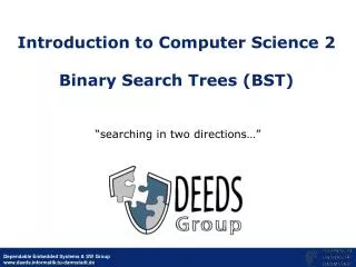
Introduction to Computer Science 2 Lecture 8: Binary search trees. “searching in two directions…”. Binary Search Tree. Root. 30. 10. 35. 1. 20. 28. 21. Binary search trees. A binary search tree is a tree where every node has at most two children Each node stores a key and some value

E N D
Introduction to Computer Science 2 Lecture 8: Binary search trees “searching in two directions…”
Binary Search Tree Root 30 10 35 1 20 28 21
Binary search trees • A binary search tree is a tree where every node has at most two children • Each node stores a key and some value • The value can also be a more complex structure or pointer • Key values are respectively unique and are elements of a totally ordered set • The order is typically numerical or lexicographical • For each node N and its left and right children L and R: • KL < KN < KR • Condition on key values permits • efficient searching • sequential and ordered processing of the data (traversal in in-order)
Definition • Already noted: Binary trees have good access costs while searching • But: While constructing binary trees, they can degenerate to a linear list (is true for binary search trees too) • The possible degeneration is the cost for having simple construction operations (no costs for rearrangement) • A native binary search tree has no rearrangement operations • Definition: A native binary search tree T is a binary tree; it is either empty or each node in T contains a key, so that: • all keys in the left subtree of T are less than the key of the root of T • all keys in the right subtree of T are greater than the key of the root of T • the left and right subtrees of T are native binary search trees too
Basic operations • Basic operations on a binary search tree: • Insert • Delete • Search for a key K • Sequential processing of all keys • Example: Insert • Binary search trees are constructed by repeatedly inserting keys • New keys are always attached to the leaves • Different sequences of insertions result in different tree structures • Procedure: • first key will be the root • all following keys are inserted recursively either in the left or in the right subtree (depending on the key values)
Java class class BinarySearchTree { int K; /* Key */ Info info; /* stored record */ BinarySearchTree L, R; /* Constructor */ public BinarySearchTree(int key, Info i) { ... } /* insert record i with key x to the tree */ public BinarySearchTree insert(int key, Info i) { ... } /* delete record with key x from the tree */ public void delete(int key) { ... } /* return node with key x if it exists, NULL otherwise */ public BinarySearchTree find(int key) { ... } /* sequential processing of all nodes in in-order */ public void inOrder( ) { ... } /* other methods ... */ }
Insert operation /* return reference to the new node, which is inserted */ public BinarySearchTree insert(int key, Info i) { if ( key < this.K ) { /* insert in the left subtree */ if ( this.L == null ) { this.L = new BinarySearchTree( key, i ); return this.L ; } else return ( this.L.insert( key, i ) ); /* Recursion */ } else { /* this.K < key , insert in the right subtree */ if ( this.R == null ) { this.R = new BinarySearchTree( key, i ); return this.R ; } else return ( this.R.insert( key, i ) ); /* Recursion */ } }
ORY ZRH JFK MEX BRU ARN DUS ORD GLA NRT GCM Example • Sequence of inserts: ORY, JFK, BRU, DUS, ZRH, MEX, ORD, NRT, ARN, GLA, GCM
GLA ORY ARN MEX ZRH BRU DUS ORD JFK NRT GCM Example (2) • Sequence of inserts: GLA, ARN, ORY, BRU, DUS, ZRH, MEX, ORD, NRT, JFK, GCM
Example (5) • Sequence of inserts: ARN, BRU, DUS, GCM, GLA, JFK, MEX, NRT, ORD, ORY, ZRH • Sorted sequence results in a degenerated tree ARN BRU DUS GCM GLA JFK MEX NRT ORD ORY ZRH
Analysis • Within n keys there are n! permutations, so n! different sequences of inserts. • Not all of them result in different trees. • Example: BRU, ARN, DUS and BRU, DUS, ARN • The number of the different native binary search trees is ( ) 1 2n n n + 1
Search (recursive) • Searching for a key is similar to inserting one • Unsuccessful search can be considered as "finding the insert position" /* return reference to the node we are searching for or NULL */ BinarySearchTree find ( int key ) { if ( this.K == key ) return this; if ( key < this.K ) { /* search in the left subtree */ if ( this.L == null ) return null; else return this.L.find( key ); } else { /* this.K < key, search in the right subtree */ if ( this.R == null ) return null; else return this.R.find( key ); } }
Search (iterative) • Searching corresponds to walking along a specific path in the tree (in the worst case starting from root to a leaf), so it doesn’t need any stack and can be implemented iteratively and efficiently. BinarySearchTree find ( int key ) { BinarySearchTree root = this; while ( root null && root.K key ) { if ( key < root.K ) root = root.L; else root = root.R; } /* now we have either root == NULL or root.K == key */ return root; }
Sequential processing • Processing of all keys in sorted order can be achieved by an in-order traversal of the tree • Ascending key values by LWR tree walk • Descending key values by RWL tree walk • Threads can in this case obviously enhance the efficiency of the operation
Delete • Delete of a node with key x is the most complicated operation. • We differentiate between three case: • Case 1: Node x is a leaf: The leaf can be deleted. There is no need for additional operations. y y z x z • Case 2: • Node x has an empty right/left subtree: delete node x, set the reference to the unique subtree of x. x z z Tl Tr Tl Tr
Delete • Case 3: Node x has two non empty subtrees: Search either for the smallest right (sr) descendent or for the greatest left (gl) descendent. Replace x with sr or gl and delete sr respectively gl from its original position. • This can be seen as switching place of x and sr (or gl) and doing delete for leaves
Delete • Delete can be performed immediately (eager strategy) or delayed (lazy) • With lazy, deleted nodes are only marked as deleted and removed later (garbage collection). • Nodes, which are marked as deleted can, if needed, be reused (if the same key is reinserted) • Deleting with an eager strategy is more complex than within a lazy • Lazy search is more complex than eager (nodes, which are marked as deleted, have also to be treated)
Example: case 1 Delete GCM GLA ORY ARN MEX ZRH BRU DUS ORD JFK NRT GCM ORY ARN MEX ZRH BRU DUS ORD JFK NRT
Example: case 2 Delete BRU: ORY ARN MEX ZRH BRU DUS ORD JFK ORY ARN MEX ZRH DUS ORD JFK
Example: case 3 GLA Two possibilities within deleting MEX result in: ORY ARN MEX BRU ZRH DUS ORD JFK GLA NRT GCM ORY ARN JFK GLA ZRH BRU ORY ARN DUS ORD NRT ZRH BRU NRT GCM DUS ORD JFK GCM
Costs of the basic operations • Which costs do the operations in a tree with n nodes have? • Sequential processing is already identified as O(n) (with different constant factors) • Costs of delete of a node x: • If x is a leaf or has an empty subtree, the costs are bounded by the depth of x • If not, the node, which will replace x, have to be found. The costs of this operation are bounded by the height of the tree • Direct search is the most important operation, since it is the basis for inserting and deletion • Search costs are in the worst case the costs for traversing the tree from the root to a leaf • Costs are bounded by the height of the tree • Search will be further investigated because of its importance
Average access costs • Possible measures (consider first successful search): • Number of accesses to the nodes (Z) • Number of key comparisons (C) • Average number of accesses can be determined over the internal path length PL(K) of the tree: • Assumption: Uniformly distributed access probability • PL(T) = i = 1 ... n depth(Ki) • Average path length L = PL(T)/n • Within each path, the root is taken into account, thus: • Zavg = L + 1
ORY ZRH JFK MEX BRU ARN DUS ORD GLA NRT GCM Example • Zavg = PL(T)/n + 1 = 3.54 accesses • Since per access two comparisons are needed (by the last/successful one only one), • Cavg = 2•Zavg - 1 = 6.08 comparisons Internal path length PL(T) = 0 + 1 + 1 + 2 + 2 + 3 + 3 + 3 + 4 + 4 + 5 = 28 n = 11
Average cost for unsuccessful search • For unsuccessful search the sum of the path lengths to “NULL” pointers is the decisive factor • Determine first the extended binary tree T’ to the tree T and then the external path length Ext of T’ • For the example: Ext = PL(T) + 2n = 50 • Assumption: Accesses to “NULL” pointers are uniformly distributed • Average number of comparisons of the unsuccessful search: C’avg (n) = 2 Ext / (n+1) • In the example: C’avg = 250 / 12 = 8.33 comparisons.
Maximum average of access costs • The longest paths (and consequently the maximum costs) result in the case of binary search trees degenerated to lists. • Height h = Lmax • At each level there is only one node, i.e., ni = 1 for all i • Zavg,max = (1/n) i = 0 ... n-1 ( i + 1 )•1 • = ½ (n + 1) O(n) • For degenerated trees the search costs are linear to the number of nodes
Average access costs • Minimum access costs can be expected in a balanced tree structure • Optimal: complete tree, h=log2(n+1) Zavg,min O(log2 n) • (Nearly) balanced tree: h=log2n+1 Zavg,minO(log2 n) • Using the formula for average path length (and some maths): • Zavg,min = log2n - 1 • Minimum and maximum average access costs are extreme values and not particularly meaningful • n = 106: • Zavg,min = 19 and Zavg,max = 500000 • The gain in average search cost is only about 40% for balanced trees!
Average access costs • First observation: avoid degenerated trees! • Significant measure: (general) average access costs • If the average access costs are close to the minimum average of access costs, the tree structure is OK • Otherwise, the tree should be rearranged • More precisely the problem is: Determining the average access costs Zavg,n as average value over all n keys and all n! search trees • Assumption: uniformly distributed access probability