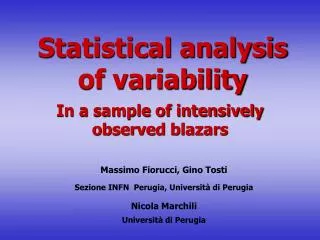
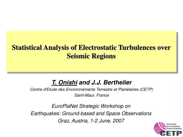
Statistical Analysis of Electrostatic Turbulences over Seismic Regions

1. Statistical Analysis of Electrostatic Turbulences over Seismic Regions T. Onishi and J.J. Berthelier Centre d'Etude des Environnements Terrestre et Planétaires (CETP) Saint-Maur, France EuroPlaNet Strategic Workshop on Earthquakes: Ground-based and Space Observations Graz, Austria, 1-2 June, 2007

2. OUTLINE • Purpose of this study • Frequency Classification of power spectra of ELF/VLF emissions • Interferences from other instruments (ISL) • Selection of Earthquake data • Preliminary results. • Conclusion and Future Work

3. TYPICAL CHARACTERISTICS OF WAVES DETECTED BY ICE Log(μV2/Hz) Ordinary ELF hiss Electrostatic Turbulance ELF hiss below Cross-over freq. ΩH+

4. Purpose of study ICE level-1 VLF spectra data with characteristic frequencies (ΩH+, etc…) calculated from IAP data. Purpose: characterize the shape of the frequency spectra to determine emissions with different origin, propagation condition etc… Track the characteristics of these emissions to search for changes linked with seismic activity. ΩH+

5. Purpose of study ICE level-1 VLF spectra data with characteristic frequencies (ΩH+, etc…) calculated from IAP data. Purpose: characterize the shape of the frequency spectra to determine emissions with different origin, propagation condition etc… Track the characteristics of these emissions to search for changes linked with seismic activity. It is easy to do it on just one spectral plot. But, there are ten of thousands of them. ΩH+

6. Automatic identification of characteristic frequencies---- Procedure ---- Savitzky-Golay smoothing  ”pwr_smooth” “Minimum” filter in time Digitalization of “pwr_smooth”  ”pwr_smooth_bin” Detection of characteristic frequencies on “pwr_smooth” from ”pwr_smooth_bin”

7. Automatic identification of characteristic frequencies---- “minimum” filter in time domain ----

8. Automatic identification of characteristic frequencies2. Smoothing in frequency domain : Savitzky-Golay filter

9. Automatic identification of characteristic frequencies2. Smoothing in frequency domain

10. Automatic identification of characteristic frequencies2. Smoothing in frequency domain : Digital filter Reduces number of candidate points and makes it easy to pick one

11. Automatic identification of characteristic frequencies2. Smoothing in frequency domain

12. So the analytical tool is ready!

13. So the analytical tool is ready! We can start the statistical study, using actual earthquake data!

14. So the analytical tool is ready! We can start the statistical study, using actual earthquake data! To begin with, let us see the electrostatic turbulence at low frequency.

15. So the analytical tool is ready! We can start the statistical study, using actual earthquake data! To begin with, let us see the electrostatic turbulence at low frequency. But…. We have a problem !!!.

16. Interferences due to the swept Langmuir probe ISL

17. Interferences due to the swept Langmuir probe ISL • Parasites are present in the form of modulation  Why? Burst mode

18. Interferences due to the swept Langmuir probe ISL • Parasites are present in the form of modulation  Why? • Knowledge of the waveform of a parasite is not enough to separate parasites from the natural emissions. (Nonlinear effects)  Only Burst Mode Burst mode

19. Interferences due to the swept Langmuir probe ISL • Parasites are present in the form of modulation  Why? • Knowledge of the waveform of a parasite is not enough to separate parasites from the natural emissions. (Nonlinear effects)  Only Burst Mode • Removal of parasite signals is very critical for the analysis of low frequency emissions (i.e. Electrostatic turbulences)  Detection and removal of parasites Burst mode

20. WHY MODULATION?

21. Parasite position inside a packet Why modulation ? VLF power spectra and waveform with Blackmann-Harris window ULF potential variations (S1 and S2) VLF power spectra obtained from VLF waveform VLF waveform and time-average

22. Parasite position inside a packet Why modulation ? VLF power spectra and waveform with Blackmann-Harris window ULF potential variations (S1 and S2) VLF power spectra obtained from VLF waveform VLF waveform and time-average

23. Parasite position inside a packet Why modulation ? VLF power spectra and waveform with Blackmann-Harris window ULF potential variations (S1 and S2) VLF power spectra obtained from VLF waveform VLF waveform and time-average

24. Parasite position inside a packet Why modulation ? VLF power spectra and waveform with Blackmann-Harris window ULF potential variations (S1 and S2) VLF power spectra obtained from VLF waveform VLF waveform and time-average

25. Parasite position inside a packet Why modulation ? VLF power spectra and waveform with Blackmann-Harris window ULF potential variations (S1 and S2) VLF power spectra obtained from VLF waveform VLF waveform and time-average

26. Parasite position inside a packet Why modulation ? VLF power spectra and waveform with Blackmann-Harris window ULF potential variations (S1 and S2) VLF power spectra obtained from VLF waveform VLF waveform and time-average

27. Parasite position inside a packet Why modulation ? VLF power spectra and waveform with Blackmann-Harris window ULF potential variations (S1 and S2) VLF power spectra obtained from VLF waveform VLF waveform and time-average

28. Why modulation ? • Voltage sweep of Langmuir probe is performed every ~1.0112 second. • Exact duration of one packet is 0.0512 second. • Relative time position voltage drop inside a packet is periodic in every 4 times.

29. We understand why parasites show a modulation.

30. We understand why parasites show a modulation. Now how can we remove them?

31. How to detect a parasite position Potential peak position is not precise enough to define the corresponding potential drop. Peak of the sweep is detected first. A point where a potential decreases by 1/e are detected on both S1. Parasite position is defined as the mid point of these two.

32. Removal of parasite signals from VLF waveform data and construction of clean VLF power spectra

33. Removal of parasite signals from VLF waveform data and construction of clean VLF power spectra

34. Removal of parasite signals from VLF waveform data and construction of clean VLF power spectra 40 spectra averaged with parasites 40 spectra averaged except those with parasites

35. After the voltage change in a potential sweep Sweep voltage is reduced from 7.6V to 3.8V from Orbit 2154.0. Parasite effect is also reduced. But……

36. After the voltage change in a potential sweep But with different contour levels, the parasite effect is evident. Parasite effects may be small. But changes due to EQs may be smaller. Such tiny changes can be masked by parasites. Therefore, parasite removal is important for low frequency analysis!

37. Now we have a tool and clean data.

38. Now we have a tool and clean data. We can start the statistical study with actual EQ data.

39. Now we have a tool and clean data. We can start the statistical study with actual EQ data. But… which EQ data can we use?

40. Now we have a tool and clean data. We can start the statistical study with actual EQ data. But… which EQ data can we use? A bunch of earthquakes often occurs in the sameregion and at about the same time (few days difference)

41. Now we have a tool and clean data. We can start the statistical study with actual EQ data. But… which EQ data can we use? A bunch of earthquakes often occurs in the same region and at about the same time (few days difference) If we should find an anomaly before one earthquake, How do we know if it is a precursor to the earthquake Or a post-seismic phenomenon of another earthquake?

42. Earthquake selection • Defining M as the magnitude of the main earthquake, following conditions are checked in EQ selection. • All EQs of magnitude smaller than M-2 are ignored. • No EQs within the dobrovolny distance of the main EQ in the preceding 10 days. • Number of EQs selected is in total 664. • M > 7.0 : 4 • 6.0 < M < 6.9 : 27 • 5.0 < M < 5.9 : 633

43. First attempt to statistical study of electrostatic turbulenceSelection Criteria • Earthquakes of magnitude 5.4 ≤ M ≤ 5.9 are used. There are 169 earthquakes. • Orbit data are used if … • In Burst mode, • ap-index ≤ 15, • -40 < Latitude < 40, • No MTB activation, • Within 200km from the epicenter In total, 59 orbits for 32 earthquakes remained.

44. First attempt to statistical study of electrostatic turbulenceFirst Result : Power Spectre at 20Hz Time (day) relative to EQ

45. First attempt to statistical study of electrostatic turbulenceFirst Result : Power Spectre at 20Hz Example with 4 EQ data sets and 7 orbits

46. First attempt to statistical study of electrostatic turbulenceFirst Result : Power Spectre at 20Hz Time (day) relative to EQ

47. First attempt to statistical study of electrostatic turbulenceFirst Result : Frequency for log(power) = -2.0 Time (day) relative to EQ

48. First attempt to statistical study of electrostatic turbulence First Result : Frequency for log(power) = -2.0 Time (day) relative to EQ

49. Better conditions: Ap-index < 10. Magnitudes 5.0 < M and Satellite distance < 100km Time (day) relative to EQ