Download
1 / 26
260 likes | 405 Vues
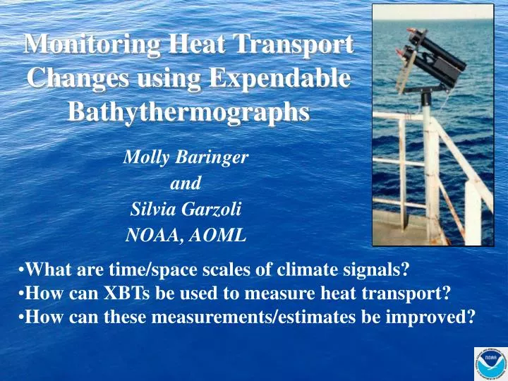
Monitoring Heat Transport Changes using Expendable Bathythermographs. Molly Baringer and Silvia Garzoli NOAA, AOML. What are time/space scales of climate signals? How can XBTs be used to measure heat transport? How can these measurements/estimates be improved?. Map of net surface heat flux.

E N D
Monitoring Heat Transport Changes using Expendable Bathythermographs Molly Baringer and Silvia Garzoli NOAA, AOML • What are time/space scales of climate signals? • How can XBTs be used to measure heat transport? • How can these measurements/estimates be improved?
Time scales of heat transport variability Short time scales: 0.9 PW over months Long time scales: 0.6 PW over decades Meridional Heat Transport 25N Time series of modeled meridional heat transport in the Atlantic. Häkkinen et al (1999) 45N
Methodology Direct estimates of lateral volume (V), mass (M) and heat (H) transport across a vertical section require T, S and velocity observations: Uncertainty in v. ?? Wind products Reference level
XBT data is collected using Sippican T-7 probes typically to depths of about 800 meters • Data is extended to the ocean bottom using Levitus 2001 data set.
Salinity in the upper ocean is estimated for each XBT by using Salinity and Temperature relationships at different locations and depths using • ARGO and CTD • Levitus 2001 climatology Temperature Salinity
Transports were computed in layers and summed for the entire water column. The level of no motion velocity was adjusted so that the net mass transport across the section was zero using a single velocity correction for each section. Typically, values of this velocity ranged from 10-4 to 10-6 m s-1. • Additional corrections/constraints to the net transports were made to account for barotropic currents: • Florida Current (Ax7) • Brazil/Malvinas Currents (Ax18) • and • Ax18 XBT sections that terminated before fully crossing the entire ocean basin.
Ekman transports: were determined using climatological wind fields interpolated to the location of the XBT lines.
Special Constraints applied to subtropical North Atlantic Section: Ax7 Winds: Hellerman and Rosenstein climatological annual mean Initial Reference Velocity: no motion along = 27.6 kg/m3 (~1000m) Boundary Currents: +32.1 Sv in the Florida Straits (long-term cable transport average)
North Atlantic Results Summary: Ax7 • Mean Heat transport from 1995 to present: • 1 PW +/- 0.2 PW • Interannual variability range: • 0.4 +/- 0.2 PW or 35% of total • Annual cycle range: • 0.1 +/- 0.2 PW or 10% of total
Methodology Error Bars? Tested Against 24N Full Water Column CTD Sections • Levitus Salinity for upper 850m: • 0.0075 +/- 0.045 PW • Levitus S(p) , T(p) below 850m: • -0.0075 +/- 0.1109 PW • Both: • 0.035 +/- 0.136 PW
Special Constraints used for South Atlantic Ax18 Winds: NCEP mean monthly values V at the bottom: Peterson (1989): Malvinas Current -0.04 m/sec at 38°S Currents on the shelf: results from Palma et al., 2004 (< 0.2 Sv)
Annual Cycle: Ax18 Ekman Heat Transport (PW): NCEP Monthly Climatology Values are ±0.2 0.7 PW) 0.8 PW 0.7 PW 0.9 PW 0.7 PW 0.8 PW 0.5 PW) 0.9 PW 0.7 PW Febr 05
Methodology Error Bars?Method tested against A10 WOCE CTD section • Unlike the North Atlantic, Levitus T(p), S(p) below 850m produces a mean bias: • +0.2 PW Bias • Still left with wind errors and other unknown variability • +/- 0.2 PW
Summary for South Atlantic: Ax18 MERIDIONAL HEAT TRANSPORT= 0.7 ± 0.2 PW BIAS due to using Levitus below 800m of0.2 PW 0.5 ± 0.2 PW
What we need to improve these estimates: • Additional constraints to improve initial estimate of total velocity field and its error covariances. • Deeper observations (fast-deep T5 to 2000+ meters?) • Specific transport estimates (e.g. Malvinas Current): XCPs? • Improved Salinity estimation (ARGO/XCTDs?) • Improved wind products and ship based observations • Improved subsurface climatologies (ARGO?) • Formalized procedure including error estimates (Inversion?)
Summary • XBTs show mean heat transports similar to historical estimates • In the North Atlantic, there has been a pronounced decrease in heat transport over the past 10 years. • More sections, improved data are necessary to determine meaningful error estimates. • Until an improved system is established, data from the high density lines can be used to obtained an estimate of the heat transport variability.