Download
1 / 26
810 likes | 1.84k Vues
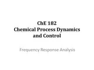
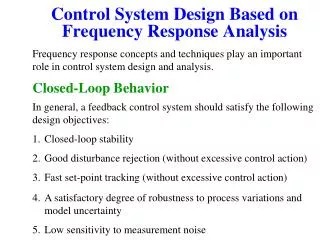
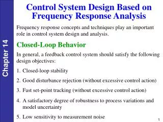
Lecture 6: Frequency Response Analysis and Stability. Objectives. To study system stability in the frequency domain using the Bode stability method. To understand the concepts of gain and phase margins. Frequency Response: determines the response of systems variables to a sine input.

E N D
Lecture 6: Frequency Response Analysis and Stability
Objectives • To study system stability in the frequency domain using the Bode stability method. • To understand the concepts of gain and phase margins.
Frequency Response: determines the response of systems variables to a sine input. Why do we study frequency response? • Perfect sine disturbances occur frequently in plants • We use sine to characterize time-varying inputs, specially disturbances • We can learn useful generalizations about control performance and robustness. No! Yes! Yes!
Frequency Response : Sine in sine out • How do we calculate the frequency response? • We could use dynamic simulation • - Lots of cases at every frequency • - Can be done for non-linear systems • For linear models, we can use the transfer function • - Remember that the frequency response can be calculated by setting s = j , with = frequency and j = complex variable.
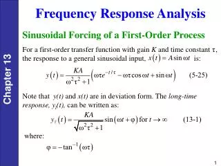
0.4 0.2 Y, outlet from system 0 -0.2 -0.4 0 1 2 3 4 5 6 time 1 0.5 X, inlet to system 0 -0.5 -1 0 1 2 3 4 5 6 time Frequency Response : Sine in sine out Amplitude ratio = |Y’(t)| max / |X’(t)| max Phase angle = phase difference between input and output P B output P’ A input
Frequency Response : Sine in sine out Amplitude ratio = |Y’(t)| max / |X’(t)| max Phase angle = phase difference between input and output These calculations are tedious by hand but easily performed in standard programming languages. In most programming languages, the absolute value gives the magnitude of a complex number.
Frequency response of mixing tank. Time-domain behavior. • Bode Plot - Shows • frequency response for • a range of frequencies • Log (AR) vs log() • Phase angle vs log()
0.8 0.6 0.4 0.2 20 0 v1 0 -0.2 0 20 40 60 80 100 120 -20 TC 100 -40 0 20 40 60 80 120 v2 STABILITY No! or Yes! We influence stability when we implement control. How do we achieve the influence we want?
1 1 0.5 0.5 0 0 -0.5 -0.5 -1 -1 1.5 1.5 0 0 0.5 0.5 1 1 First, let’s define stability: A system is stable if all bounded inputs to the system result in bounded outputs. Sample Inputs Sample Outputs Process bounded bounded unbounded unbounded
STABILITY The denominator determines the stability of the closed-loop feedback system! Set point response Bode Stability Method Calculating the roots is easy with standard software. However, if the equation has a dead time, the term e -s appears. Therefore, we need another method. The method we will use next is the Bode Stability Method.
SP(s) E(s) CV(s) MV(s) + + GC(s) Gv(s) GP(s) + - CVm(s) Loop open GS(s) Bode Stability: To understand, let’s do a thought experiment
No forcing!! No forcing!! SP(s) SP(s) E(s) E(s) CV(s) CV(s) MV(s) MV(s) + + + + GC(s) GC(s) Gv(s) Gv(s) GP(s) GP(s) + + - - CVm(s) CVm(s) Loop closed Loop closed GS(s) GS(s) Bode Stability: To understand, let’s do a thought experiment Under what conditions is the system stable (unstable)? Hint: think about the sine wave as it travels around the loop once.
SP(s) E(s) CV(s) MV(s) + + GC(s) Gv(s) GP(s) + - CVm(s) Loop closed GS(s) Bode Stability: To understand, let’s do a thought experiment If the sine is larger in amplitude after one cycle; then it will increase each “time around” the loop. The system will be unstable. Now: at what frequency does the sine most reinforce itself?
SP(s) E(s) CV(s) MV(s) + + GC(s) Gv(s) GP(s) + - CVm(s) Loop closed GS(s) Bode Stability: To understand, let’s do a thought experiment When the sine has a lag of 180° due to element dynamics, the feedback will reinforce the oscillation (remember the - sign). This is the critical or phase crossover frequency, pc.
Bode Stability Let’s put the results together. GOL(s) includes all elements in the closed loop. At the critical frequency: GOL(pcj) = -180 The amplitude ratio: |GOL(pcj) | < 1 for stability |GOL(pcj) | > 1 for instability The gain margin (GM) is define as: GM = Hence, if the gain margin is less than 1 (negative in dB), the system is unstable.
Phase Margin Another relevant term is the phase margin. To calculate it, we need to find the gain crossover frequency(gc) whichis the frequency at which the open-loop gain crosses unity. The phase margin (PM) is the distance between the open loop phase and -180 at frequency gc PM = If the phase margin is negative, the system is unstable.
Interpretation of Gain and Phase Margins • The gain margin tells us the maximum proportional gain we are allowed to use without affecting system stability. • The phase margin tells us the maximum additional phase (and also dead time) that can be added to the loop without affecting system stability. The best way to understand these two points is to try a numerical example!
Example Find the gain and phase margin for the following process under proportional control. Is the system stable? . Find the delay margin as well.
Answer • To find the gain margin, we need the phase crossover frequency. . • This gives rad/sec. • At this frequency, = (system stable) dB. • Therefore, the gain margin = 1/0.735 = 1.36 = 2.63 dB.
Answer • To find the phase margin, we need the gain crossover frequency. . • This gives rad/sec. • At this frequency, = --2tan-1() = -1-2tan-1(1) = - 1 - = -2.57 rad = -147.3.
Answer • Therefore, the phase margin (PM) = + = 0.57 rad = 32.7. • The delay margin, DM = = = 0.57 sec.
We can check our result using the command “margin” in Matlab. s=tf(‘s’); G=2/(s+1)^2*exp(-s); margin(G)
Let us now use Simulink to understand the interpretation of gain margin and phase margins. • For this purpose, we build the following model:
Closed-loop step response (original process with proportional controller gain = 1) The system is stable.
Closed-loop step response with proportional controller of gain 1.4. The system is unstable. Remember that the gain margin is 1.36.
Closed-loop step response with proportional controller of gain 1 and additional delay of 0.6 sec. Remember that the phase margin tells us that additional delay must not exceed 0.57. The system is unstable.