Download
1 / 7
210 likes | 1.38k Vues
Translog Cost Function. E. Berndt and D. Wood, "Technology, Prices, and the Derived Demand for Energy," Review of Economics and Statistics , 57, 1975, pp 376-384 . Production and Cost Functions. Production function: Q = f( x ) Cost minimizing factor demands: x i = x i (Q, p )

E N D
Translog Cost Function E. Berndt and D. Wood, "Technology, Prices, and the Derived Demand for Energy," Review of Economics and Statistics, 57, 1975, pp 376-384.
Production and Cost Functions • Production function: Q = f(x) • Cost minimizing factor demands:xi = xi(Q,p) • Cost function: C = Si=1,…M pixi(Q,p) = C(Q,p)
Theory of Cost Function • Shephard’s Lemma: xi = xi(Q,p) = C(Q,p)/pipixi/C = (pi/C) C(Q,p)/pi • Factor Shares: si = lnC(Q,p)/ lnpi • Elasticity of Factor Substitution: • (Own and Cross) Price Elasticity:
Theory of Cost Function • Constant returns to scale: C = Qc(p) • Average cost function: c(p) = C/Q • Marginal cost function: C/Q = c(p) • Linear homogeneity in prices: lc(p)=c(lp) • 2nd order Taylor approximation of lnc(p) at lnp = 0:
Berndt-Wood Model • U.S. Manufacturing, 1947-1971 • Output and Four Factors: Q, K, L, E, M • Prices: PK, PL, PE, PM • The constant return to scale translog cost function:ln(C) = b0 + ln(Q) + bKln(PK) + bLln(PL) + bEln(PE) + bMln(PM) + ½ bKKln(PK)2 + ½ bLLln(PL)2 + ½ bEEln(PE)2 + ½ bMMln(PM)2 + bKLln(PK)ln(PL) + bKEln(PK)ln(PE) + bKMln(PK)ln(PM) + bLEln(PL)ln(PE) + bLMln(PL)ln(PM) + bEMln(PE)ln(PM) • Symmetric conditions: bij = bji, i,j = K,L,E,M
Berndt-Wood Model • Factor shares:SK = PKK/C, SL = PLL/C, SE = PEE/C, SM = PMM/C SK+SL+SE+SM = 1 (because PKK+PLL+PEE+PMM = C) • Factor share equations: SK = bK + bKK ln(PK) + bKL ln(PL) + bKE ln(PE) + bKM ln(PM)SL = bL + bKL ln(PK) + bLL ln(PL) + bLE ln(PE) + bLM ln(PM)SE = bE + bKE ln(PK) + bLE ln(PL) + bEE ln(PE) + bEM ln(PM)SM = bM + bKM ln(PK) + bLM ln(PL) + bEM ln(PE) + bMM ln(PM) • Elasticities:qij = bij/(SiSj) + 1 if i≠j; qij = bij/(SiSi) + 1 - 1/Si, hij = Sjqij, i,j=K,L,E,M
Berndt-Wood Model • Linear restrictions:bK + bL + bE + bM = 1bKK + bKL + bKE + bKM = 0 bKL + bLL + bLE + bLM = 0bKE + bLE + bEE + bEM = 0bKM + bLM + bEM + bMM = 0 • Stata programs and datasets: • bwp.dta, bwq.dta • bw1.do, bw2.do, bw3.do