Download
1 / 8
90 likes | 199 Vues
Chapter 4. How fast is the simplex method. Efficiency of an algorithm : measured by running time with respect to the problem size. Two models of computation time: arithmetic operation model: assumes each operation (addition, multiplication, …) takes unit time.

E N D
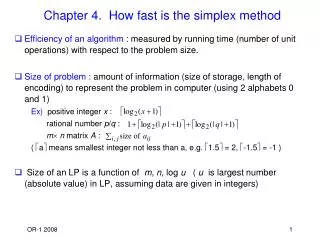
Chapter 4. How fast is the simplex method • Efficiency of an algorithm : measured by running time with respect to the problem size. • Two models of computation time: • arithmetic operation model: assumes each operation (addition, multiplication, …) takes unit time. • bit operation model: counts the number of “bits operations”. depends on the sizes of numbers written in binary notation. • Size of problem : amount of information (size of storage, length of encoding) to represent the problem in computer (using 2 alphabets 0 and 1) Ex) positive integer : rational number : m n matrix A : ( means smallest integer not less than , e.g. , ) • Size of an LP is a function of ( is largest number (absolute value) in LP, assuming data are given in integers)
Running time : worst case view point • An algorithm is considered efficient if the worst case running time is bounded from above by a polynomial function of problem size (for large instances only, small instances can be solved fast anyway). (called polynomial time algorithm) Running time Size of problem encoding
function is called (is read big oh of ) if there exist a positive constant and a positive integer such that when . e.g.) • Why polynomial function? Suppose it takes 1 sec in running time when , then • Suppose one iteration of simplex method takes polynomial time of the input size (which is true). Then, if the number of iterations is a polynomial function of input length for any LP, it implies that simplex method is a polynomial time algorithm.
Empirically, the number of iterations is and • Bad counter example : Klee and Minty (1972) maximize subject to , , If we use largest coefficient rule, number of iterations is , hence running time is not polynomial
ex) max s.t. Note that , and feasible region is given approximately as Hence it is an elongated skewed hypercube with extreme points. (Note that we need 3 equations to define an extreme point in this example. Only one of the lower and upper bound constraints for each variable can be chosen to define an extreme point, hence total of extreme points exist.) • Simplex method with largest coefficient rule searches all extreme points until it finds the optimal solution. But, largest increase rule finds the optimal solution in one iteration.
largest increase rule • Geometric view
Alternative rules : Largest increase rule : counter example by Jeroslow (1973) Bland’s rule : counter example by Avis and Chvatal (1978) Hence, until now, simplex method is not a polynomial time algorithm theoretically. But it performs very well practically. • First polynomial time algorithm for LP : ellipsoid method (1979) by L. G. Khachian. But, practically much inferior to simplex. However, it has some important theoretical implications in determining computational complexity of some optimization problems. • Another polynomial time algorithm : Interior point method by L. Karmarkar (1984) : Better than simplex in many cases practically. Many versions. Based on ideas from nonlinear programming.
Interior point method will be briefly mentioned when we study complementary slackness theorem. • Comparing simplex and interior point method: Interior point method is generally fast, especially for large problems. But simplex is competitive for some problems and recent developments in dual simplex algorithm makes solving LP of large size manageable. In addition, simplex is effective when we solve the LP again after making some changes in data (reoptimization). Such capability is quite important when we solve integer programming problems. But little progress has been made for interior point algorithm in this respect. Recently, interior point method is used for some nonlinear programming problems (convex programs) with successful results.