Download
1 / 68
700 likes | 1.19k Vues
Binary Trees, Binary Search Trees, and AVL Trees. This is a PowerPoint slideshow with extensive animation; it is meant to be viewed in slideshow mode. If you’re reading this text, you’re not in slideshow mode. Enter slideshow mode by hitting function key 5 on your keyboard (the F5 key).

E N D
Binary Trees,Binary Search Trees, and AVL Trees This is a PowerPoint slideshow with extensive animation; it is meant to be viewed in slideshow mode. If you’re reading this text, you’re not in slideshow mode. Enter slideshow mode by hitting function key 5 on your keyboard (the F5 key) The Most Beautiful Data Structures in the World • This animation is a PowerPoint slideshow • Hit the spacebar to advance • Hit the backspace key to go backwards • Hit the ESC key to terminate the show
A D P W C L F T E J M K V AVL Trees: Motivation AVL trees, named after the two mathematicians Adelson-Velsky and Landis who invented/discovered them, are of great theoretic, practical, and historic interest in computer science as they were the first data structure to provide efficient — i.e., O(lg n) — support for the big three of data structure operations: search, insertion, and deletion The proof of their O(lg n) behavior illuminates the complex and beautiful topological properties that an abstract data structure can have This presentation provides an overview of that proof — along with a decent review of some of the basics of binary trees along the way
A D P W C L F T E J M K V Roadmap • Binary trees in general • Definitions, vocabulary, properties • The range of possible heights for binary trees (and why we care) • Binary search trees • The search (or find) algorithm • Insertion • Deletion • The problem (or why we need AVL trees) • AVL trees • Definition: An HB(1) binary search tree • O(1) rebalancing to restore the HB(1) property after the BST insertion • Finding the deepest node out of balance in O(h) time • Proof that the HB(1) property means that h is O(lg n) • Some engineering implications of AVL tree properties
Binary Trees A binary tree is an abstract data structure that is either empty or has a unique root with exactly two subtrees, called the left and the right subtrees, each of which is itself a binary tree (and so may be empty) Here are illustrations of some typical binary trees: A binary tree having a root with two empty subtrees The empty binary tree Note that this is a different binary tree than the one to the left The root in this one has an empty left subtree but a non-empty right one A binary tree having a root with a non-empty left subtree and an empty right subtree Doesn’t look particularly “binary”, but it’s still a binary tree — just one with every node having an empty right subtree Note that the definition for a binary tree is recursive — unlike trees from graph theory which are defined based on graph theoretic properties alone (no recursion) Thus it is technically correct to say that a binary tree is not a graph and hence is not really a tree no one but me ever says that anymore; but although it’s not particularly important, it’s still the truth, so I want you to know it
level # 0 1 2 3 4 5 h=5 Properties and Nomenclature of Binary Trees and Nodes Every node except the root has a unique parent Nodes can be categorized by level, starting with the root at level 0 The left (or right) child of a given node plus all that child’s descendants are collectively referred to as the left (or right) descendants of the original node The highlighted subtree contains the left descendants of this node A node with two children is said to be full A full binary tree is one where all internal nodes are full — so there are no nodes with just one child, everybody is either a leaf or full Although this particular node is full, the tree here is not A node is the parent of its children This node has a left child but no right child This node also has a sibling, a node with the same parent The height of a node is the path length to its deepest descendant This node has height 2 There are many additional topologic properties (also called “shape” properties) that we’ll be defining and working with, such as the relationship between a binary tree’s height and its number of nodes, which we’ll examine next A node with no descendants is called an external or leaf node A node with descendants is called an interior or internal node A node may or may not have descendants; but every node except the root has one or more ancestors The height of a binary tree is the depth of its deepest node; so this binary tree has a height of 5 • Two more or less obvious consequences of this definition: • The height of any leaf is 0 • The height of the root is the height of the whole tree The depth of a node is its level number; which is the number of edges (path length) between the node and the root This node is at level 4 and so has a depth of 4 We’ll often use genealogical terminology when referring to nodes and their relationships Topologic properties of nodes and trees will be important too
A D P W C L F T E J M K V Roadmap • Binary trees in general • Definitions, vocabulary, properties • The range of possible heights for binary trees (and why we care ;-) • Binary search trees • AVL trees
Range of Possible Heights for Binary Trees (and Why We Care) • The height and number of nodes in a binary tree are obviously related • For any given number of nodes, n, there is a minimum and a maximum possible height for a binary tree which contains that number of nodes – e.g., a binary tree with 5 nodes can’t have height 0 or height 100 • Contra wise, for any given height, h, there is a minimum and maximum number of nodes possible for that height – e.g., a binary tree with height 2 can’t have 1 node or 50 nodes in it • We’re very interested in the minimum and maximum possible heights for a binary tree because when we get to search trees (soon) it will be easy to see that search and insertion performance are O(h); the tougher question will be, what are the limitations on h as a function of n? • Large h leads to the poor performance • Small h will result in good performance
n=4, h=3 Maximum Possible Height It’s easy to see that the greatest possible height for a binary tree containing n nodes is h=n-1 • For maximum height, we want the maximum number of levels, so each level should contain the fewest possible nodes — which is to say 1, since a level cannot be empty • So the tallest tree having n nodes would have n levels • The largest level # would then be n-1, since we start numbering levels with the root at level 0 • So the maximum height for a binary tree containing n nodes is h=n-1 The minimum possible height (the best case for O(h) performance) is a bit more interesting
Two Necessary Definitions Along the Way(to the Minimum Possible Height for a Binary Tree) • Note: • If we add another node to this almost perfect tree, there’s only one place it could go and still keep the tree almost perfect by keeping the bottom level all left justified • So for any given number of nodes, n, there is only one almost perfect binary tree with n nodes — the shape is unique • Since the shape is unique, the best case and worst case heights are the same: Given a number of nodes, n, there’s only one possible height for an almost perfect binary tree of that given number of nodes A perfect binary tree has the maximum possible number of nodes at every level To reduce the height of this almost perfect binary tree, all the nodes here at the bottom would have to go into a higher level somewhere; but they can’t — by definition, all the upper levels already contain their maximum possible number of nodes An almost perfect (also known as complete) binary tree has the maximum number of nodes at each level except the lowest, where all the nodes are “left justified” An almost perfect binary tree is the most compact of all binary trees, it has the minimum possible height for its number of nodes So to know the minimum possible height for any binary tree of n nodes, all we have to do is figure out the (unique) height of an almost perfect binary tree with n nodes
level 0 has 20 =1 nodes level 1 has 21= 2 nodes level 2 has 22 = 4 nodes level 3 has 23= 8 nodes level 4 has 24= 16 nodes level k has 2k nodes The number of nodes in a binary tree (any binary tree) is obviously the sum of the number of nodes in all its levels, so a perfect binary tree with height h, which has levels 0 through h, has a total number of h k=0 nodes n = lk, where lkis the number of nodes at level k = 2k =2h+1-1 h k=0 • • • Total Number of Nodes in a Perfect Binary Tree • Note that a perfect binary tree is also a full binary tree • Every interior node has 2 children • If there were an interior node that didn’t have 2 children, the level beneath it would not have the maximum possible number of nodes • Since all internal nodes are full and there are no leaves except at the bottom level, each level has twice as many nodes as the one above it Although what we’re really after is the height of an almost perfect binary tree, we need to know the number of nodes in a perfect binary tree first (trust me on this ;-)
h-1 h Height of an Almost Perfect Binary TreeSpecial Case Consider first the special case of an almost perfect binary tree whose bottom level has only a single node in it The rest of this tree above the bottom level is obviously a perfect binary tree of height h-1 Since this “upper” portion is a perfect binary tree of height h-1, it has2k = 2(h-1)+1 -1 = 2h-1 nodes h-1 k=0 So, adding in the single node at the bottom level, in this special case n = 2h nodes Taking the binary logarithm of both sides, we get h = log2n
Height of an Almost Perfect Binary TreeGeneral Case Now the overall height has grown to h+1 which is exactly log2 n again Suppose there’s more than one node on the bottom level? h h+1 In between, as the bottom level fills up, h ≤log2n < h+1 The height h has remained the same even though log2 n has grown Butlog2 n can’t have grown as large as h+1; it won’t get that big until we fill the last level completely and have to add the next node to a new lowest level Since h is an integer, we can express h ≤ log2n < h+1 ash= log2n, where x is the “floor” function, the largest integer ≤ x The equality occurring, of course, only when we have only a single node at the bottom level
log2n ≤h≤ n-1 This is the height of an almost perfect binary tree with n nodes, which shape we know has the minimum possible height for any binary tree This is the height of the maximally “stretched out” shape we looked at earlier Range of Possible Heights, h, for Binary Trees with n Nodes So when we show that some binary tree operation is O(h), which we can often do rather easily, we’ll know that it’s either O(lg n) or O(n) or somewhere in between Since that can make a pretty big difference in actual performance, the hard work will come in trying to figure out which end we’re at, O(lg n) or O(n), and figuring out ways to drive it down towards O(lg n)
A D P W C L F T E J M K V Roadmap • Binary trees in general • Binary search trees • Definitions and the search (or find) algorithm • Insertion • Deletion • The problem (or why we need AVL trees) • AVL trees
? ? Insertion Into a Binary Tree There’s no obvious rule to tell us where to insert a new node into a binary tree in general There would seem to be lots of possibilities; we’ll need some additional property that we wish to preserve to help us decide For (somewhat silly) example, if we were trying to preserve a “zig-zag” shape property, this spot would be the only place we could insert the next node and still have a zig-zag tree ? ? ? For our discussion of AVL trees, the binary search tree property is the one we’re interested in
L M F T S S F K H M Here’s a binary tree with at least one node that does not obey the BST property; so this binary tree is not a BST Binary Search Trees A binary search tree (or BST) is a binary tree where each node contains some totally ordered* key value and all the nodes obey the BST property: The key values in all the left descendants of a given node are less than the key value of that given node; the key values of its right descendants are greater This binary tree is a BST … although this node is happy enough The key value here… Note that the problem is not between parent and child but between more distant, but still ancestral, relations — all the descendants of a node must have the correct key relationship with it, not just its children … causes this node to fail the BST property … * Values are totally ordered iff, for any two keys , , exacty one of three relationships must be true: < , or = , or >
T F L C W P E D J M A G K V Searching a BST to Find Some Node Given a Key <M >M We’ve fallen out of the tree; the search for a node with a key of ‘O’ was unsuccessful >J <T Find(K) K Find(O) O <L <P = The search for an existing node with a key of ‘K’ is successful • Start searching at the root of the tree and then loop as follows: • If the key we’re searching for matches the key in the current node, we’re done; the search was successful • Else if the key we want is less than the current one we’re looking at, move down to the left and try again • Else if the key we want is greater than the current one we’re looking at,move down to the right and try again • Else (when we’ve fallen out of the tree), the search was unsuccessful Searching is a fundamental data structure operation and, as we will see, is the first part of the insertion (and deletion) algorithm for a BST as well Searches are said to terminate successfully or unsuccessfully, depending on whether or not the desired node is found Performance of the search algorithm: Since we only have to check the key of one node per level, regardless of how many other nodes might be at that same level, the search time is proportional to the number of levels, which is the same as h, the height of the tree; so search time is O(h)
A D P W C L F T E J M K V Roadmap • Binary trees in general • Binary search trees • Definitions and the search (or find) algorithm • Insertion • Deletion • The problem (or why we need AVL trees) • AVL trees
L W C F T A J M P D E G K V G Simple Insertion Into a BST G<M G<J G>E Order of Insertions G>F insert(M) insert(T) insert(J) The insertion started with a standard search of a binary search tree The place where the unsuccessful search “fell out of the tree” is where the new node must be inserted so as to preserve the BST property So insertion, like search, is clearly O(h) insert(W) insert(L) insert(P) Insertion into a BST involves searching the tree for the empty place (found by an unsuccessful search) where the new node needs to go if the BST property is to be preserved The BST above was built by the sequence of insertions shown to the left Let’s look at the details of the next insertion insert(V) insert(E) insert(C) insert(F) insert(K) insert(D) insert(A) insert(G)
A D P W C L F T E J M K V Roadmap • Binary trees in general • Binary search trees • Definitions and the search (or find) algorithm • Insertion • Deletion • The problem (or why we need AVL trees) • AVL trees
A D P W C L F T E J M K V Deletion From a Binary Search Tree • Deletion from a BST takes two steps: • Find the node to be deleted using the standard search/find algorithm • Delete it and rebuild the BST as necessary • Nothing new in the first step, so let’s assume we’ve done that and consider the three cases that are needed to cover the second step: • The node to be deleted has no children • The node to be deleted has only one child • The node to be deleted has two children
A D P W C L F T E J M K V Deletion of a Node With No Children As a programming matter, you’d probably want to have saved that old pointer value somewhere first, before setting it to NULL so you could, for example, return unused storage to the operating system via a call to the freefunction But as far as the BST itself is concerned, the deletion merely requires setting the correct parent pointer to NULL To delete a node with no children, the correct pointer from its parent is just set to NULL and poof, the node has been deleted
parent of deleted node D k1 k2 A P T C L E J M W node to be deleted promoted child only child of node to be deleted K V descendants (if any) of promoted child Deletion of a Node With Only One Child Only one link needed to change to delete the desired node and promote its child Let’s delete node ‘L’ Note that the BST property is preserved by the promotion: No left or right ancestor-descendant relationships are altered anywhere Specifically, the now promoted child and all its descendants (if any) remain to the same side of the parent of the now deleted node as they were before the deletion In this example, node ‘K’ and its descendants were to the right of node ‘J’ before the deletion of node ‘L’ and they are to the right of node ‘J’ after the deletion and their subsequent promotion To delete a node with only one child, the child is “promoted” to replace its deleted parent All the promoted child’s descendants (if any) move up with it and so will be unaffected by the deletion of one of their ancestors
node to be deleted C A D P W L F F J M ? E T K V J K L Deletion of a Node With Two Children … so as to ensure that the BST property holds between the newly promoted node and its left descendents … and move up here … Deleting a node with 2 children is going to take some more work (and some thinking first ;-) … or it comes from somewhere on the right Either the replacement comes from somewhere on the left of the node being deleted … If, for example, we promote node ‘F’, we will have destroyed our BST – nodes, ‘J’, ‘K’, and ‘L’ are greater than ‘F’ but would be to its left Let’s look at the case where it comes from the left – the other case is just the reverse Once we have found the node to be deleted, we have easy access to its descendants but, unless we’ve done something special, we have no access to its ancestors (if any – here, for example, we’ll delete the root) So what we want to do is replace the data in the node being deleted with data from one of its descendents, so none of the deleted node’s ancestors need to be changed The question of whom to promote is not as obvious as it was for the case where it just had a single child Whichever node we choose to “promote” from here … So any node from the left of the node we’re deleting will be OK for promotion as far as preserving the BST property with regard to all the nodes on the right of the node being deleted But how about the promoted node’s relationship with the other nodes still remaining on the left after its promotion? So in order to preserve the BST property here in the left subtree, the node we choose to “promote” has to be the one having the largest key value … … will by the definition of a BST have a key less than that in any node here There are two choices for where to find the replacement node to promote and either one will actually work just fine
node with largest key value in left subtree of node being deleted node being deleted W A D F C P E J L ? T K V Finding the Largest Node in the Left Sub-tree Is Pretty Simple, Actually Move down to the left once (to get to the root of the left subtree) … … which brings us to the node with the largest key value in the left sub-tree of the node to be deleted … and then slice* down to the right (to bigger and bigger key values) until reaching a node with no right child … ______________________ *slice: keep moving in the same direction (down-right, in this case)until you can’t go any farther in that direction
node just promoted A D P W C F T E J L K V Oops! We just “orphaned” the promoted node’s child! But this problem will be easier to fix than you might think
node just promoted J T F C L P D A E W K V Lr Ll Orphans Yucko! After promotion of the orphan, the BST has been restored There would appear to be the standard three possibilities: • There are no orphans; it (node ‘L’) actually had no children (node ‘K’ never existed), in which case after promoting node ‘L’ we’re all done, the BST property holds everywhere • It had exactly one child, as in the example shown here; in which case the orphaned child itself (node ‘K’) and its descendants (if any) can be promoted a single level, as we saw on an earlier chart • It (node L) had two children (Ll to the left and Lrto the right) and we have to go through this whole process all over again since we just effectively deleted a node with two children! When will it ever end? But the yucko 3rd case, two children, can’t happen! The node just promoted, ‘L’, couldn’t have had two children (Lland Lr) or it wouldn’t have had the largest key in the subtree(Lrwould be greater) and so it, node ‘L’, wouldn’t have been selected for promotion in the first place – node ‘Lr’ would have been selected for promotion Q.E.D
A D P W C L F T E J M K V Summary of Deletion From a Binary Search Tree • Deletion from a BST takes two steps: • Find the node to be deleted using the standard search/find algorithm • Delete it and rebuild the BST as necessary • Three cases for the second step • The node to be deleted has no children • The node to be deleted has only one child • The node to be deleted has two children – the BST can be rebuilt by promoting the node with the largest key value from its left subtree or the node with the smallest key value from its right subtree • It’s easy enough to show that all three cases are still O(h)
A D P W C L F T E J M K V Roadmap • Binary trees in general • Binary search trees • Definitions and the search (or find) algorithm • Insertion • Deletion • The problem (or why we need AVL trees) • AVL trees
W T M V So What’s the Problem? An arbitrary series of insertions and deletions can produce a “skinny” BST where h = n-1, leading to a BST for which search and insertion, which are always O(h), are therefore O(n), not the O(lg n) we want This is in fact a real BST, albeit it a “skinny” one that doesn’t look particularly “binaryish” insert(M) insert(T) insert(W) insert(V) The problem is that we need the almost perfect shape, or something very similar, with h = log2 n, to get the O(h) performance to be O(lg n) But our insertion algorithm did not consider shape at all in determining where to insert a new node; so in general, unless we get lucky, we won’t wind up with an almost perfect shape after we do an insertion “No problem”, you say; first, we’ll do the simple insertion and then afterwards rebuild the almost perfect shape Unfortunately, the “rebuilding” could easily be Ω(n), hardly what we want
M F T B M C H F T H B C The Almost Perfect Shape is The ProblemIt’s Too Stringent, Too Expensive to Maintain Note that every single parent-child relationship had to be changed to restore the BST property, an Ω(n) operation at best ! Here’s an almost perfect binary search tree with n=5 nodes After we rebuild to almost perfect shape, it will have to look like this … And here’s the only possible arrangement of the nodes that ensures the BST property is preserved for the new almost perfect BST … since there’s only one possible shape for an almost perfect binary tree with 6 nodes And here’s the tree after the insertion of a node with the key of ‘C’ It’s still a BST, but it’s no longer almost perfect
Conclusions (vis a vis Binary Search trees) Although BST insertion is O(h) and an almost perfect shape guarantees that h=log2n, we can’t usually keep the almost perfect shape after a BST insertion without rebuilding, an operation that can often be Ω(n), which surely defeats the goal of making the complete insertion operation itself O(lg n) The almost perfect shape constraint is the problem; it’s too difficult to maintain — i.e., it usually can’t be done O(lg n) What we need is an “easier” shape constraint, one that can always be restored with just O(lg n) operations after an insertion The shape constraint we’re after is called the “height bounded with differential 1” or HB(1) property; and it’s what makes AVL trees possible
C F L E W T D A J M P G K V Roadmap • Binary trees in general • Binary search trees • AVL trees • Definition: An HB(1) binary search tree • O(1) rebalancing to restore the HB(1) property after the BST insertion • Finding the deepest node out of balance in O(h) time • Proof that the HB(1) property means that h is O(lg n) • Some engineering implications of AVL tree properties
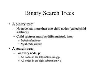
J L C R F W A P W B D I J L V M M E T F T G K V P AVL Trees: BSTs With the HB(1) Property An AVL tree is a binary search tree in which each node also obeys the HB(1) property: The heights of its left and right subtrees must differ by no more than 1 Both the BST and HB(1) properties must hold for every node The tree above is an AVL tree The tree to the right is a BST that is not HB(1) and so is not an AVL tree This node, F, is not in HB(1) balance
A D P W C L F T E J M G K V Insertion Into an AVL Tree Insertion into an AVL tree occurs in two steps: • Do a normal BST insertion so as to preserve the BST property without regard for the HB(1) property • Determine if the BST insertion broke the HB(1) property anywhere, and, if so, fix it somehow while satisfying two constraints: • The fixing operation must be O(lg n) or better • The fixing operation must preserve the BST property
nodes now out of balance L F C A M D E T P W J G K V B J M An HB(1) Breaking Insertion B<M B<J B<E Order of Insertions B<C insert(M) B>A insert(T) insert(J) insert(W) insert(L) insert(P) insert(V) Although it naturally preserved the BST property, this last insertiondestroyed the HB(1) balance of multiple nodes We’re going to need to restore the HB(1) balance somehow The AVL tree above was built from an initially empty tree by the sequence of BST insertions shown to the left This sequence was carefully chosen so that the insertions never broke the HB(1) property anywhere We won’t always be so lucky; let’s try another insertion insert(E) insert(C) insert(F) insert(K) insert(D) insert(A) insert(G) insert(B)
E L A D B P J M T C F W G B M J HB(1) Re-Balancing:Key Nodes and Subtrees deepestnode out of balance nodes now out of balance left child of deepest node out of balance newleft sub-tree of left child of deepest node out of balance old left sub-tree of left child of deepest node out of balance #3 K V #2 #1 last insertion For the left-left case, three subtrees are the key to a re-arrangement that will restore the HB(1) balance to all nodes currently out of balance without disturbing the binary search tree property anywhere, thus restoring the AVL tree: The example here is a left-left case, one where the destructive insertion occurred under the left subtree of the left child of the deepest node now out of balance #1is the (new) left subtree of the left child of the deepest node out of balance There are three other similar cases (left-right, right-left, and right-right) #2is the right subtree of the left child of the deepest node out of balance #3is the right subtree of the deepest node out of balance These three subtrees’ heights always have a fixed relationship to each other that is central to correcting the imbalance induced by the last insertion
J M A D T C E P L F W G h h h h+1 B M J Height Analysis of the Three Subtrees deepestnode out of balance left child of deepest node out of balance #3 K V subtree #3also has height exactly h • If subtree#3had height < h, the deepest node out of balance would have been out of balance before the last insertion • If subtree#3had height >h, the deepest node allegedly out of balance would not, in fact, be out of HB(1) balance at all, and that would be a contradiction #2 subtree #2must be height h, the same height assubtree#1 was before the last insertion: • If subtree#2had height <h, the left child of the allegedly deepest node out of balance would itself be out of HB(1) balance and that would be a contradiction • If subtree#2had height>h,the deepest node out of balance would have been out of HB(1) balance before the last insertion #1 The last insertion changed the height of subtree#1fromhto h+1, and, in so doing, destroyed the HB(1) balance of one or more of its ancestors If the height of subtree#1 hadn’t changed, no nodes would be out of balance In this particular example, h=1; but in general, h can be any integer 0, depending on the topology of the tree at the time of the destructive insertion Summary: In the left-left case, subtrees #2 and #3 have to be the same height, which must be exactly one less than the height of subtree #1 Reminder: h can be any integer 0, depending on the shape of the original tree and where the last insertion took place
A D B F C T E W P L M J #3 G K h h h+1 h+1 #1 M J Re-Balancing the AVL Tree With a Rotation V #2 Because of the fixed relationship among the heights of the three subtrees, the whole AVL tree can be rebalanced after a left-left case insertion by “rotating” subtrees#1 and #3 around subtree#2 three links Only needed to be changed to achieve the rotation to restore the HB(1) balance for the entire tree It doesn’t matter if there are a gazillion nodes in subtrees #1, #2, and #3; it’s still only three links that need to be changed to restore the HB(1) property; so the rotation is an O(1) operation Note that the binary search tree property has been preserved
T L P W J M F D B C E A G The Rebalanced AVL Tree V K Each node still has the binary search tree property Each node is now again in HB(1) balance
Summary So Far • The example showed the rotation for the left-left case – the insertion that destroyed the HB(1) balance somewhere was at the bottom of the left sub-tree of the left child of the deepest node that wound up out of balance • A right-right case is obviously the mirror image of some left-left case • The left-right and right-left cases each require two rotations to rebalance the tree, not just one, but each rotation is still a fixed number of steps, i.e., they’re still O(1)
So … After an O(h) BST insertion into an HB(1) binary search tree, the HB(1) balance can be restored while preserving the binary search tree property with at most two O(1) rotations Doing the rotation(s) is just O(1), but how do we find the deepest node out of balance, which is the key to the rotation?
A D P W C L F T E J M K V Roadmap • Binary trees in general • Binary search trees • AVL trees • Definition: An HB(1) binary search tree • O(1) rebalancing to restore the HB(1) property after the BST insertion • Finding the deepest node out of balance in O(h) time • Proof that the HB(1) property means that h is O(lg n) • Some engineering implications of AVL tree properties
M M J C A E J E C A B B 0 0 1 1 0 2 0 1 3 4 1 0 0 0 3 0 1 0 2 0 0 0 1 0 2 0 Only nodes that are ancestors of the node just inserted need to be checked for HB(1) balance after an insertion Nothing changed in any subtree of any non-ancestral node ; they were in balance before, so they’re still in balance now Finding the Deepest Node Out of Balance B<M B<J B<E B<C These are the subtree heights from before the last insertion, we’re about to look at the algorithm that adjusts them B>A the top of the stack is the parent of the node just inserted Note that the stack, LIFO data structure that it is, has “inverted” the levels of the ancestors — nodes higher in the stack are actually from deeper in the original tree So the first time we pop the stack and discover an ancestor out of balance, it is the deepest node out of balance We’ll also need to provide two extra data fields in each node to allow us to keep track of its subtrees’ heights, which we’ll use to determine balance, if and when we insert underneath it If we push onto a stack the nodes we check on the way down to find the insertion point, we’ll have a data structure that contains the only nodes we need to check for HB(1) balance the stack here’s the root of the whole tree
After the insertion, we’ll start popping the stack to access the next ancestor up from the node just inserted and check and adjust its subtree heights as necessary Whenever we pop a node, we know that it was HB(1) before the last insertion, so there are only two possibilities for the relationship between the heights of its left and right subtrees before the last insertion: They were equal: or The ancestor had a short and a long side, differing in height by 1: The left or right locations of the tall side and the short side of these icons, above, are irrelevant to the concepts here; although they’re relevant to the actual code we’d have to write, all we care about for our conceptual proof here is that the ancestor’s subtree heights were unequal (but obviously differed by only 1) M J E C A Using the Stack to Process the Ancestors From the Bottom Up or the stack
A C E J M the ancestor just popped off the stack, HB(1) before the last insertion the node just inserted While the Stack Is Not Empty • Pop an ancestor node off the stack • Check the popped node for one of three cases: • Its previously short side grew taller • One of its two previously equal sides grew taller • Its previously long side grew taller a subtree prior to the last insertion
We’re all done: there’s nothing more to be checked or modified. All nodes above this current node retain the HB(1) left and right subtree heights they had before the insertion Case 1: Short-Side Grew Taller current node whose subtree heights are to be examined and updated We have to record, in the current (just popped) node, a new subtree height for one of its subtrees, since the height of its previously short-side subtree just increased by 1 h-1 h Note that the overall height of the tree rooted at the current node has not changed; it was h before; it’s still h now Ergo: None of the heights of any subtrees of any ancestors of the current node have changed either
Again, we have to record that the height of one of the subtrees of the current node has just increased by 1 Although the current node remains HB(1), its overall height has increased by 1, so the height of some subtree of its parent has also increased by 1; so we’ll have to continue on up the tree, popping the stack and processing the next ancestor up (the parent of the current node) If the stack is empty, of course, the current node we’ve just finished processing is the root of the original tree, in which case we’re all done: the last insertion did not destroy the HB(1) balance anywhere and we have correctly updated all affected nodes’ subtree heights Case 2: A Previously Equal Height Subtree Grew Taller current node whose subtree heights are to be examined and updated Note that the overall height of the tree rooted at the current node has changed h h+1
deepest node out of balance this node is now out of balance h h+1 h+2 Case 3: Long-Side Grew Taller current node whose subtree heights are to be examined and updated Before the last insertion, the difference between the heights of the two subtrees of the current ancestor was 1 After the insertion, the difference between the heights of the subtrees is now 2 Since we built the stack on the way down, as we searched for our insertion point, nodes higher in the stack were deeper in the tree, so the first time we pop a node from the stack and discover that it is out of balance, it is the deepest node out of balance
out of balance ancestor to deepest node out of balance deepest node out of balance T W A T J M J L W L P A D C E D F E C P B #3 G G K V last insertion K #1 B J Case 3: Long-Side Grew Taller (cont’d) M M 4 3 F V Before the last insertion (that destroyed its balance), the height of the left subtree of this node was 4, which is no longer the case But after the rotation, this height for the left subtree is correct again Since neither of the subtree heights for this temporarily out of balance node had to be changed, nothing needs to be checked or changed in any of its ancestors (if any) either #2 And the deepest node out of balance is the only one we care about! We don’t need to continue to look for othernodes out of balance farther up the tree: Even if such nodes exist, the rotation we’re about to do with the just identified deepest node out of balance will restore the balance for any higher out of balance nodes as well,and leave their old values for their subtree heights correct and unchanged So once we do the rotation, we’re all done; the tree is rebalanced and each node’s recorded subtree heights are correct