Download
1 / 27
280 likes | 403 Vues
Lattice QCD + Hydro/Cascade Model of Heavy Ion Collisions. Michael Cheng Lawrence Livermore National Laboratory. 2010 Winter Workshop on Nuclear Dynamics Ocho Rios, Jamaica, January 2-9, 2010. Outline. Calculation of T c via lattice QCD – domain wall fermion method

E N D
Lattice QCD + Hydro/Cascade Model of Heavy Ion Collisions Michael Cheng Lawrence Livermore National Laboratory 2010 Winter Workshop on Nuclear Dynamics Ocho Rios, Jamaica, January 2-9, 2010
Outline • Calculation of Tc via lattice QCD – domain wall fermion method • Parameterization of LQCD EoS • Model of heavy ion collision including: • Initial, non-equilibriumflow (Pratt) • 2D viscuous hydrodynamics (Romatschke’s vh2) • Parton cascade (URQMD)
Staggered • Many recent high-precision calculations are performed with some variant of staggered fermiondiscretization (stout-link, asqtad, p4, HISQ) • Single quark flavor for staggered fermions correspond to 4 flavors of continuum quark flavor. • Spontaneous breakdown of SU(4) chiral symmetry -> 15 Goldstone bosons. • However, lattice effects explicitly break SU(4) chiral symmetry -> U(1). Only one GB. Other pions have non-zero mass of O(a2) • To recover a one flavor theory on the lattice, take ¼ root.
Domain Wall Fermions • Domain Wall Fermions (DWF) faithfully preserve SU(Nf) chiral symmetry to arbitrary accuracy even at finite lattice spacing. • Therefore, meson spectrum, e.g. 3 light pions, is more correctly reproduced by DWF method. • Penalty: QCD with DWF is recovered as a 4-d space-time slice of a 5-d theory.
Staggered v. DWF • Primary reason to use staggered fermions: cost. • Size of fifth dimension in DWF calculations: 8-32. • Staggered fermions approach smaller lattice spacing at high precision faster than DWF. • Since T = 1/(Nta), lattice calculations are done at fixed Nt and varying lattice spacing. • Until recently, onlylargelattice spacingsfeasiblefor exploration of finite T QCD (Nt=4, 6). In this regime, DWF formulation does not work so well
DWF at Nt = 8 • Well-known disagreement for Tc among staggered fermion calculations. Cannot agree on whether chiral, deconfining transitions are distinct. Tc = 150-200 MeV • Calculations at Nt=8 for DWF are feasible. Useful check on the staggered calculations. • Work done in collaboration with RBC Collaboration (arXiv:0911.3450) • Vary lattice coupling (β=6/g2) to change temperature. • Calculate chiral, deconfinement observables.
χl/T2 -> Chiral susceptibility. Peaks in transition region • Δl,s/T3 -> Chiral condensate. Non-zero at low temperature, zero at high temperature.
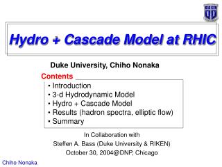
Deconfinement observables: isospin and charge susceptibilities. • Inflection point determined by fitting data to ansatz. • Consistent with peak in chiral susceptibility. • However, SB limit already saturated at low temperature, as expected as DWF formulation is unimproved at high temperature.
Caveats • Limitations in this calculation: • Small volume (Finite volume effects not controlled) • Lacks precision of staggered studies. • Quark mass not held constant in this calculation -> mπ ≈ 300 MeV at T = 170 MeV, but larger at low temperature, smaller at high temperature. • Single lattice spacing – cannot make continuum extrapolation (4-7% error suggested by other calculations) • Single set of masses – guess at extrapolation to physical quark masses.
Comparison with Ls = 96 calculation Preliminary! Tc = 171(17)(10)MeV
Description of Model • Hybrid model includes: • Pre-thermalization flow (Pratt arXiv:0810.4325) • 2D viscuous hydrodynamic evolution (Romatshke’s vh2) • Hadron cascade, afterCooper-Fryefreezeout (URQMD) • Examine the effect of varying: • Equation of state (LQCD EoS vs. 1st order transition) • Viscosity • Pre-thermalization flow. • Initial conditions/freezeout temperature • Collaborators: • Ron Soltz, Andrew Glenn, Jason Newby (LLNL and ORNL) • Scott Pratt • Talk by R. Soltz at CATHIE/TECHQM
Parameterizing LQCD EoS • Already saw a more detailed study in talk by Petreczky, but also many others. • Let f(T) be parameterization of EoS • Suggestion by K. Rajagopal: • 1/f(T) = 1/g(T) + 1/h(T) • g(T) -> low temperature • h(T) -> high temperature • h(T) = d2/T2 + d4/T4 • g(T) = (a + (T/T0)b)*HRG(T) • Fix low T to HRG by setting a = 1.0 PRD 80, 014504 2009
Description of existing runs • Initial Flow • From Glauberprofile. • b= 3.4, 5.5 fm., Tinitial = 250-350 MeV • Vh2 2-D hydro: • η/s = 0.08 – 0.40 • EoS = RomatchskeEoS, LQCD, LQCD+HRG • Cooper-Frye freezeout • Tfreezeout= 120 – 170 MeV • URQMD for hadroniccascade • Match spectra to tune parameters
Conclusions • Calculation of crossover temperature with DWF to compare with staggered-type calculations. • Tc~ 170 MeV, but with large error because of statistics and several systematic uncertainties. • No splitting evident for deconfinement, chiral observables • Not really in disagreement with either of conflicting staggered calculations. • Exploratory calculation – need to do a calculation that corrects many of the flaws of current calculation. • One is underway, thinking about other methods, but still computationally too expensive…
Conclusions (cont.) • Hybrid model including pre-thermalization flow + 2D viscuous hydrodynamics + URQMD (almost) working. • Still work in progress. • Goals: • Study collective flow, femtoscopy. • Effects of varying η/s, initial conditions, Tfreezeout • Does pre-thermal flow help explain HBT puzzle? • Quantify effects of varying EoS • Systematic comparison to experimental data.