Download
1 / 28
280 likes | 284 Vues
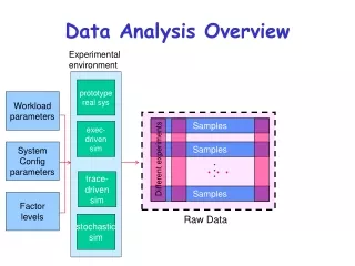
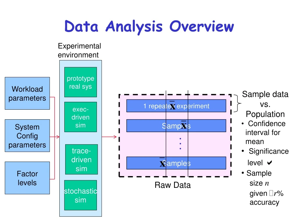
Sample data vs. Population Confidence interval for mean Significance level a Sample size n given ! r % accuracy. Data Analysis Overview. Experimental environment. prototype real sys. Workload parameters. _. x. 1 repeated experiment. exec- driven sim. _. x.

E N D
Sample data vs.Population • Confidence interval for mean • Significance level a • Sample size ngiven !r% accuracy Data Analysis Overview Experimentalenvironment prototype real sys Workloadparameters _ x 1 repeated experiment exec-drivensim _ x SystemConfigparameters Samples ... trace-drivensim _ x Samples Factorlevels Raw Data stochasticsim
Confidence Intervals • Sample mean value is only an estimate of the true population mean • Bounds c1 and c2 such that there is a high probability, 1-a, that the population mean is in the interval (c1,c2): Prob{ c1 < m < c2} =1-awhere a is the significance level and100(1-a) is the confidence level • Overlapping confidence intervals is interpreted as “not statistically different”
Confidence Intervalof Sample Mean • Knowing where 90% of sample means fall, we can state a 90% confidence interval • Key is Central Limit Theorem: • Sample means are normally distributed • With population mean • With standard deviation (standard error) • If observations in sample are independent and come from population with mean and s.d.s
EstimatingConfidence Intervals • Two formulas for confidence intervals • Over 30 samples from any distribution: z-distribution • Small sample from normally distributed population: t-distribution • Common error: using t-distribution for non-normal population
The z Distribution • Interval on either side of mean: • Significance level is small for large confidence levels • Tables of z are tricky: be careful!
Example of z Distribution • 35 samples: 10 16 47 48 74 30 81 42 57 67 7 13 56 44 54 17 60 32 45 28 33 60 36 59 73 46 10 40 35 65 34 25 18 48 63 • Sample mean = 42.1. Standard deviation s = 20.1. n = 35 • 90% confidence interval is
The t Distribution • Formula is almost the same: • Usable only for normally distributed populations! • But works with small samples
Example of t Distribution • 10 height samples: 148 166 170 191 187 114 168 180 177 204 • Sample mean = 170.5. Standard deviation s = 25.1, n = 10 • 90% confidence interval is • 99% interval is (144.7, 196.3)
Getting More Confidence • Asking for a higher confidence level widens the confidence interval • Counterintuitive? • How tall is Fred? • 90% sure he’s between 155 and 190 cm • We want to be 99% sure we’re right • So we need more room: 99% sure he’s between 145 and 200 cm
Making Decisions • Why do we use confidence intervals? • Summarizes error in sample mean • Gives way to decide if measurement is meaningful • Allows comparisons in face of error • But remember: at 90% confidence, 10% of sample means do not include population mean
Testing for Zero Mean • Is population mean significantly nonzero? • If confidence interval includes 0, answer is no • Can test for any value (mean of sums is sum of means) • Example: our height samples are consistent with average height of 170 cm • Also consistent with 160 and 180!
Comparison of Alternatives • Paired Observations • As one sample of pairwise differences ai - bi • Confidence interval A B . . . Data Analysis Overview Experimentalenvironment prototype real sys Workloadparameters 1 experiment exec-drivensim SystemConfigparameters Samples 1 set of experiments ... trace-drivensim Samples Factorlevels Raw Data stochasticsim
Unpaired Observations • As multiple samples, sample means and overlapping CIs • t-test on mean difference: xa - xb xb , sb ,CIb xa , sa ,CIa . . . Data Analysis Overview Experimentalenvironment prototype real sys Workloadparameters 1 experiment exec-drivensim SystemConfigparameters Samples 1 set of experiments ... trace-drivensim Samples Factorlevels Raw Data stochasticsim
Comparing Alternatives • Often need to find better system • Choose fastest computer to buy • Prove our algorithm runs faster • Different methods for paired/unpaired observations • Paired if ith test on each system was same • Unpaired otherwise
Comparing Paired Observations • Treat problem as 1 sample of n pairs • For each test calculate performance difference • Calculate confidence interval for differences • If interval includes zero, systems aren’t different • If not, sign indicates which is better
Example: Comparing Paired Observations • Do home baseball teams outscore visitors? • Sample from 9-4-96:
Example: Comparing Paired Observations • H-V 2 -2 -7 5 6 -1 -7 6 7 3 2 1 -1 6 • Mean 1.4, 90% interval (-0.75, 3.6) • Can’t reject the hypothesis that difference is 0. • 70% interval is (0.10, 2.76)
B B B mean mean mean A A A Comparing Unpaired Observations • A sample of size na and nb for each alternative A and B • Start with confidence intervals • If no overlap: • Systems are different and higher mean is better (for HB metrics) • If overlap and each CI contains other mean: • Systems are not different at this level • If close call, could lower confidence level • If overlap and one mean isn’t in other CI • Must do t-test
The t-test (1) 1. Compute sample means and 2. Compute sample standard deviations saand sb 3. Compute mean difference = 4. Compute standard deviation of difference:
The t-test (2) 5. Compute effective degrees of freedom: 6. Compute the confidence interval: 7. If interval includes zero, no difference !
! Comparing Proportions • Categorical variables • If k of n trials give a certain result, then confidence interval is • If interval includes 0.5, can’t say which outcome is statistically meaningful • Must have k>10 to get valid results
Special Considerations • Selecting a confidence level • Hypothesis testing • One-sided confidence intervals
Selecting aConfidence Level • Depends on cost of being wrong • 90%, 95% are common values for scientific papers • Generally, use highest value that lets you make a firm statement • But it’s better to be consistent throughout a given paper
Sample Sizes • Bigger sample sizes give narrower intervals • Smaller values of t, v as n increases • in formulas • But sample collection is often expensive • What is the minimum we can get away with? • Start with a small number of preliminary measurements to estimate variance.
Choosing a Sample Size • To get a given percentage error ±r%: • Here, z represents either z or t as appropriate • For a proportion p = k/n:
Example ofChoosing Sample Size • Five runs of a compilation took 22.5, 19.8, 21.1, 26.7, 20.2 seconds • How many runs to get ±5% confidence interval at 90% confidence level? • = 22.1, s = 2.8, t0.95;4= 2.132