Download
1 / 51
520 likes | 770 Vues
A Random-Surfer Web-Graph Model. (Joint work with Avrim Blum & Hubert Chan ). Mugizi Rwebangira. links.html. index.html. http://cnn.com. resume.html. The Web as a Graph. Consider the World Wide Web as a graph, with web pages as nodes and hyperlinks between pages as edges.

E N D
A Random-Surfer Web-Graph Model (Joint work with Avrim Blum & Hubert Chan) Mugizi Rwebangira
links.html index.html http://cnn.com resume.html The Web as a Graph Consider the World Wide Web as a graph, with web pages as nodes and hyperlinks between pages as edges.
Studying the Web Since the Web emerged there has been a lot of interest in: • Empirically studying properties of the Web Graph. • Modeling the Web Graph mathematically. Benefits of Generative Models: • Simulation – When real data is scarce • Extrapolation – How will the graph change? • Understanding– Inspire further research on real data
Power Law f(x) ~ g(x) if Limx→∞ f(x)/g(x) = 1 e.g (x+1) ~ (x+2) The distribution of a random variable X follows a power law if Prob [X=k]~ Ck-α Example: Prob [X=k]=k-2
Power Law Prob [X=k] ~ Ck-α log Prob [X=k] ~ log C –αlog k Prob [X=k]=k-2 log Prob [X=k]= -2 logk
Power Law contd. More general definition: Prob [X≥k]~ Ck-α Particularly useful if X takes on real values. Sometimes referred to as “heavy tailed” or “scale free.”
Power Laws inDegree distribution Let G be a graph. Let Xk be the proportion of nodes with degree k in G. Then if Xk~ Ck-α we say that G has power law degree distribution.
Properties of the Web Graph A Power-law degree distribution has been observed in a wide variety of graphs including citation networks, social networks, protein-protein interaction networks and so on. It has also been observed in the Web Graph. [Barabási & Albert]
Outline • Background/Previous Work • Motivation • Models • Theoretical results • Experimental results • Conclusions
Classic Random Graph Models • In the G(n,p) random graph model: • There are n nodes. • There is an edge between any two nodes with probability p. • Was proposed by Erdös and Renyi in 1960s.
Online G(n,p) In this model each new node makes k connections to existing nodes uniformly at random. For this talk we will focus on k = 1, hence the graph will be a tree.
T=1 T=2 T=3 ½ ½ T=4 ⅓ ⅓ ⅓ Online G(n,p)
Properties of Online G(n,p) • E[degree of first node] = 1+ 1/2 +1/3+1/4 + …1/n = (log n) • E[max degree] = (log n) • Xk = Proportion of nodes with degree k E[Xk] = (½k) NOT POWER LAWED!!
Preferential Attachment In the Preferential Attachment model, each new node connects to the existing nodes with aprobability proportional to their degree. [Barabási & Albert]
Degree = in-degree + out-degree T=1 T=2 Deg = 1 Deg = 3 T=3 ¾ ¼ T=4 Deg = 1 Deg = 4 Deg = 1 Preferential Attachment
Preferential Attachment E[degree of 1st node] = √n Preferential Attachment gives a power-law degree distribution. [Mitzenmacher, Cooper & Frieze 03, KRRSTU00]
Other Models Kumar et. al. proposed the “copying model.” [KRRSTU00] Leskovec et. al. propose a “forest fire” model which has some similarites to this work. [LKF05]
Outline • Background/Previous Work • Motivation • Models • Theoretical results • Experimental results • Conclusions
Motivating Questions • Why would a new node connect to nodes of high degree? • Are high degree nodes more attractive? • Or are there other explanations? How does a new node find out what the high degree nodes are?
Motivating Questions Motivating Observation: • Suppose each page has a small probability p of being interesting. • Suppose a user does a (undirected) random walk until they • find an interesting page. • If p is small then this is the same as preferential attachment. • What about other processes and directed graphs?
Outline • Background/Previous Work • Motivation • Models • Theoretical results • Experimental results • Conclusions
Start with a single node with a self-loop. T=1 (½) (½)+ (½) (½)+ (½) (½) • Choose a node uniformly at random • With probability p connect • With probability (1-p) connect to its neighbor T=2 T=3 ¾ ¼ Directed 1-step Random Surfer, p=.5
Directed 1-step Random Surfer It turns out this model is a mixture of connecting to nodes uniformly at random and preferential attachment. Has a power-law degree distribution. But taking one step is not very natural. What about doing a real random walk?
Directed Coin Flipping model • Pick a node uniformly at random. 2. Flip a coin of bias p If HEADS connect to current node, else walk to neighbor D C NEW NODE B A RANDOM STARTING NODE 1. COIN TOSS: TAIL (at node A) 2. COIN TOSS: TAIL (at node B) 3. COIN TOSS: HEAD (at node C)
Directed Coin Flipping model • At time 1, we start with a single node with a self-loop. • At time t, we choose a node uuniformly at random. • We then flip a coin of bias p. • If the coin comes up heads, we connect to the current node. • Else we walk to a random neighbor and go to step 3. “each page has equal probability p of being interesting to us”
Outline • Background/Previous Work • Motivation • Models • Theoretical results • Experimental results • Conclusions
Is Directed Coin-Flipping Power-lawed? We don’t know … but we do have some partial results ...
Virtual Degree Definitions: • Let li(u)be the number of levelidescendents of node u. • l1(u) = # of children • l2(u) = # of grandchildren, e.t.c. Let = (β1, β2,..) be a sequence of real numbers with 1=1. Thenv(u) = 1 + β1 l1(u) + β2 l2(u) + β3 l3(u) + … We’ll call v(u) the “Virtual degree of u with respect to .”
u v(u) = 1 + β1 (2) + β2 (4) + β3 (0) + β4 (0) + ... # of children # of grandchildren Virtual Degree
u Virtual Degree Easy observation: If we set βi = (1-p)i then the expected increase in deg(u) is proportional to v(u). Expected increase in deg(u) = p/t + (1-p)pl1(u)/t + (1-p)2pl2(u)/t + … = (p/t)v(u)
Virtual Degree • Theorem: There always exist βi such that • For i ≥ 1, |βi| · 1. • As i → ∞, βi →0 exponentially. • The expected increase in v(u) is proportional to v(u). Recurrence:1=1, 2=p, i+1=i – (1-p)i-1 E.g., for p=¾, i = 1, 3/4, 1/2, 5/16, 3/16, 7/64,... for p=½, i = 1, 1/2, 0, -1/4, -1/4, -1/8, 0, 1/16, …
Virtual Degree, continued Let vt(u) be the virtual degree of node u at time t and tu be the time when node u first appears. Theorem: For any node u and time t ≥tu, E[vt(u)] = Θ((t/tu)p) So, the expected virtual degrees follow a power law.
Actual Degree We can also obtain lower bounds on the expected values of the actual degrees: Theorem: For any node u and time t ≥tu, E[degree(u)] ≥ Ω((t/tu)p(1-p))
Outline • Background/Previous Work • Motivation • Models • Theoretical results • Experimental results • Conclusions
Experiments • Random graphs of n=100,000 nodes • Compute statistics averaged over 100 runs. • K=1 (Every node has out-degree 1)
Outline • Background/Previous Work • Motivation • Models • Theoretical results • Experimental results • Conclusions
Conclusions Directed random walk models appear to generate power-laws (and partial theoretical results). Power laws can naturally emerge, even if all nodes have the same intrinsic “attractiveness”.
Open questions • Can we prove that the degrees in the directed coin-flipping model do indeed follow a power law? • Analyze degree distribution for the undirected coin-flipping • model with p=1/2? • Suppose page i has “interestingness” pi. Can we analyze • the degree as a function of t, i and pi?