Download
1 / 6
60 likes | 166 Vues
MS698: Implementing a Hydrodynamic Model. Case Study 1: One-Dimensional Vertical Step 3: Change something and rerun the model.

E N D
MS698: Implementing a Hydrodynamic Model Case Study 1: One-Dimensional VerticalStep 3: Change something and rerun the model.
Overview ofOne-Dimensional Model “SED_TOY”Really is a small three-d model that is uniform in x, y.Uses periodic boundary conditions at x, y boundaries.The model “sed_toy” has 6 rho-points in the u-direction, 5 in the v-direction, and 20 vertical layers. Wind shear Y direction (v) Z direction (omega) Big gray arrows represent periodic boundary conditions. Blue arrows represent “v” velocities. Purple are “u” velocities. Gray x’s are the “rho points”. X direction (u) X direction (u)
Overview of ROMS Model Forcing • Specified in ocean_sedtoy.in: • Twenty vertical layers. • Time step, and length of model run. • Specified in analytical files (ana_smflux.h): • Wind stress. Originally the wind blew with a high stress for 3000 seconds, then stopped. Last week you made the wind blow continuously, but with a weaker stress. • More grid information. Bathymetry is twenty meters. • Specified in the “header” file, sed_toy.h are the model configurations. • Choice of turbulence closure. • Mode of surface and bottom boundary conditions for momentum.
Your Assignment • To finish this case study – take the model that you ran last week and choose something to change about it. • With your lab partner, make the change and rerun the model. Make sure to have output files for both the original and the revised model. • Make figures that illustrate the model output, and that compare the results from the two models. You should have at least one figure that shows a timeseries, and another one that shows a vertical profile. You can work on the figures with your partner. • On your own: Produce a 3 – 5 page (double spaced) report that describes the original model, the change that you made, and how that change influenced the model results. • Due in one week (Feb. 21).
Suggestions of Model Experiments that Might be Interesting (and work). • Change the wind stress (magnitude, direction, or timing. • Change the water depth. • Change the number of vertical layers. • Change the timestep or length of the model run. • Use a different bottom roughness. • This version neglects Coriolis. Try the model with Coriolis. • This model is running sediment resuspension. You could change the sediment properties.
Some Hints • To make figures that you can use in your report: I like to use the “print –dpng” matlab command. This creates a pngfile; for example if you want “figure1.png” you would type “print –dpng figure1”, and I think that would work. • You can also save figures as “*.fig” file using “saveas”, and then reopen it in matlab later. You would type “saveas(gcf, ‘figure1.fig’, ‘fig’)”. You can also use this command to save figures in other formats (e.g. “saveas(gcf, ‘figure1.png’, ‘png’)”. • The vertical grid of ROMS – if you change the water depth or the vertical layering you will need to recalculate the vertical grid to plot vertical profiles. • In MATLAB: z_rho=roms_depths_old(ocean_his.nc, grid.nc, ‘rho’); • Provides water depth at rho points for all time steps and spatial dimensions. • Can get this function at: /pacific/export/home2/moriarty/matlab/roms_depths_old.m • Or, a copy of the vertical grid for the original model run is saved here: /pacific/export/home2/moriarty/Class/Hydrodynamic_modeling_2014/z.mat