Download
1 / 45
450 likes | 578 Vues
Parsimony Methods. NJ was originally described as a method for approximating a tree that minimizes the sum of least-squares branch lengths – the minimum – evolution criterion.

E N D
Parsimony Methods • NJ was originally described as a method for approximating a tree that minimizes the sum of least-squares branch lengths – the minimum – evolution criterion. • However, it rarely achieves this goal for data sets of nontrivial size, and rearrangements of the NJ tree that yield a lower minimum – evolution score can usually be found. This result makes it difficult to defend the presentation of an NJ tree as the most reasonable estimate of a phylogeny.
Background • The basic idea underlying parsimony analysis is simple: one seeks the tree, or collection of trees, that minimizes the amount of evolutionary change required to explain the data. • The goal of minimizing evolutionary change is often defended on philosophical grounds. • One line of argument is the notion that when two hypotheses provide equally valid explanations for a phenomenon, the simpler one should always be preferred.
Background • To use simplicity as a justification for parsimony methods in phylogenetics, one must demonstrate a direct relationship between the number of character-state changes required by a tree topology and the complexity of the corresponding hypotheses. • Related arguments have focused on the concepts of falsifiability and corroboration most strongly associated with the writings , suggesting that parsimony is the only method consistent with a hypothetico-deductive framework for hypothesis testing.
Despite more than 20 years of ongoing debate between those who advocate the exclusive use of parsimony methods and those who favor maximum-likelihood and related model-based statistical approaches, the issue remains unsettled and the camps highly polarized. • Although we place ourselves firmly on the statistical side.
7.3 • The problem of finding optimal trees under the parsimony criterion can be separated into two subproblems: • (1) determining the amount of character change, or tree length, required by any given tree • (2) searching over all possible tree topologies for the trees that minimize this length.
For ntaxa, an unrooted binary tree, n-2 internal nodes; 2n-3 branches Where N is the number of sites (characters) in the alignment and lj is the length for a single site j. This length lj is the amount of character change implied by a most parsimonious reconstruction that assigns a character-state xij to each node input data. Thus, for binary trees:
Where a (k) and b (k) are the states assigned to the nodes at either end of branch k, andcxy is the cost associated with the change from state x to state y. • This cost is simply 1 if x and y are different or 0 if they are identical. Assign a greater cost to transversions than to transitions as a cost matrix, or step matrix, that assigns a cost for the change between each pair of character states.
In general, the cost matrix is symmetric (e.g., cAG = cGA), with the consequence that the length of the tree is the same regardless of the position of the root. If the cost matrix contains one or more elements for which cxy≠ cyx, then different rootings of the tree may imply different lengths.
In general, with an alphabet size of r (e.g., r = 4 states for nucleotides, r = 20 states for amino acids) and T taxa, the number of these reconstructions for each site is equal to rT-2. • Thus, this character does not discriminate among the three tree topologies and is said to be parsimony-uninformative under this cost scheme. With 4:1 transversion : transition weighting, the minimum length is five steps.
p.166 • Under these unequal costs, the character becomes informative in the sense that some trees have lower lengths than others, which demonstrates that the use of unequal costs may provide more information for phylogeny reconstruction than equal-cost schemes. • Summing these lengths to obtain the total tree length for each possible tree, and then choosing the tree that minimizes the total length. Obviously, for real applications, a better way is needed for determining the minimum lengths that does not require evaluation of all rn-2reconstructions.
1 ATATT 2 ATCGT 3 GCAGT 4 GCCGT
1 ATATT 2 ATCGT 3 GCAGT 4 GCCGT
7.4.1 Exact methods • For eleven or fewer taxa, a brute-force exhaustive search is feasible; an algorithm is needed that can guarantee generation of all possible trees for evaluation using the previously described methods.
An alternative exact procedure, the branch-and bound methods, is useful for data sets containing from 12 to 25 or so taxa. This method operates by implicitly evaluating all possible trees, but cutting off paths of the search tree when it is determined that they cannot possibly lead to optimal trees. • Throughout this traversal, an upper bound on the length of the optimal tree(s) is maintained.
(1) using a heuristic method such as stepwise addition or NJ to find a tree whose length provides a smaller initial upper bound, which allows earlier termination of search paths in the early stages of the algorithm; (2) ordering the sequential addition of taxa in a way that promotes earlier cutoff of paths (rater than just adding them in order of their appearance in the data matrix); and (3) using techniques such as pairwise character incompatibility to improve the lower bound on the minimum length of trees that can be obtained by continuing outward traversal of the search tree (allowing earlier cutoffs).
When data sets become too large to use the exact searching methods, it becomes necessary to resort to the use of heuristics: approximate methods that attempt to find optimal solutions but provide no guarantee of success. • stepwise addition • Unlike the exact exhaustive enumeration and branch-and –bound methods, stepwise addition commits to a path out of each node on the search tree that looks most promising at the moment. • This tendency to become “stuck” in local optima is a common property of greedy heuristics, and they are often calledlocal-search methods for that reason.
Tree-rearrangement perturbations known as branch-swapping. These methods all involve cutting off one or more pieces of a tree (subtrees) and reassembling them in a way that is locally different from the original tree. Three kinds of branch-swapping moves are used in PAUP*. • Nearest-neighbor interchange (NNI) are T – 3 internal branches. Each branch is visited.
Subtree pruning and regrafting (SPR), involves clipping off all possible subtrees from the main tree and reinserting them at all possible locations, but avoiding pruning and grafting operations that would generate the same tree.
The most extensive rearrangement strategy available in PAUP* is tree bisection and reconnection (TBR) involve cutting a tree into two subtrees by cutting one branch, and then reconnecting the two subtrees by creating a new branch that joins a branch on one subtree to a branch on the other.
s to v; s to w; s to y‘; r to v; r to w; r to y‘; y to v; y to w
(D) Bisection of branch y and reconnection of branch r to v; other TBRs would connect r to w, r to y‘;s to v, s to w, s to y‘;y to v, and y to w, respectively. • All other branches, both internal and external, also would be cut in a full round of TBR swapping.
Note that the set of possible NNIs for a tree is a subset of the possible SPR rearrangements, and that the set of possible SPR rearrangements is in turn a subset of the possible TBR rearrangements.
If a rearrangement is successful in finding a shorter tree, the previous tree is discarded and the rearrangement process is restarted on this new tree. Optionally, when trees are found that are equal in score to the current tree, they are appended to a list of optimal trees. If a rearrangement of this next tree yields a better tree than any found so far, all trees in the current list are discarded.
Hill-climbing algorithms, such as the branch-swapping methods implemented in PAUP*, are susceptible to the problem of entrapment in local optima. • One generally successful method for improving the chances of obtaining a globally optimal solution is to begin the search from a variety of starting points in the hope that at least one of them will climb the right hill. An option available in PAUP* is to start the search from randomly chosen tree topologies.
Starting branch-swapping searches from a variety of random-addition-sequence replicates thereby provides a mechanism for performing multiple searches that each begin at a relatively high point on some hill, increasing the probability that the overall search will find an optimal tree. • Random-addition-sequence searches are also useful in identifying multiple islands of trees.