Download
1 / 44
440 likes | 586 Vues
Flux Emergence & the Storage of Magnetic Free Energy. Brian T. Welsch Space Sciences Lab, UC-Berkeley Flares and coronal mass ejections (CMEs) are driven by the release of free magnetic energy stored in the coronal magnetic field.

E N D
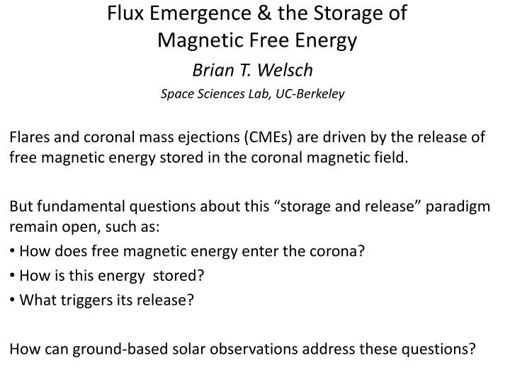
Flux Emergence & the Storage of Magnetic Free Energy Brian T. Welsch Space Sciences Lab, UC-Berkeley Flares and coronal mass ejections (CMEs) are driven by the release of free magnetic energy stored in the coronal magnetic field. But fundamental questions about this “storage and release” paradigm remain open, such as: How does free magnetic energy enter the corona? How is this energy stored? What triggers its release? How can ground-based solar observations address these questions?
Flares and CMEs are powered by energy in the coronal magnetic field. From T.G. Forbes, “A Review on the Genesis of Coronal Mass Ejections”, JGR (2000)
The hypothetical coronal magnetic field with lowest energy is current-free, or “potential.” • For a given coronal field Bcor, the coronal magnetic energy is: • U dV (Bcor·Bcor)/8. • The lowest energy coronal field would have current J = 0, and Ampére says 4πJ/c = x B, so x Bmin= 0. • A curl-free vector field can be expressed as the gradient of a scalar potential, Bmin = -. (Since ·Bmin= -2 = 0, it’s easy to solve!) • Umin dV (Bmin·Bmin)/8 • The difference U(F) = [U – Umin] is “free” energy stored in the corona, which can be suddenly released in flares or CMEs.
Coronal J cannot currently be observationally constrained; measurements of (vector) Bcor(x, y, z) haven’t been made. In consequence, we must use indirect means to infer properties of coronal currents. When not flaring, Bphotosphere and Bchromosphereare coupled to Bcor, so provide valuable insights. While Bcor can evolve on its own, changes in BphorBchwill induce changes in the coronal field Bcor. In addition, following active region (AR) fields in time can provide information about their history and development.
Unfortunately, our ignorance regarding free magnetic energy in the corona is profound! 1. Physically, how does free energy enter the corona? • Practically, how can we detect this buildup? 2. Physically, how is this energy stored? • Practically, how can we quantify it once it’s there? 3. Physically, what triggers its release? • Practically, how can we predict when release is imminent? Common theme: we want to know vectorB (so we can infer J)from the photosphere upward into the corona.
Some Key Roles for Ground Based Efforts: • Develop means to estimate vector B(x,y,z) in chromosphere and corona (radio, IR).
Short answer to #1: Energy comes from the interior!But how? EUV image of ~1MK plasma • Image credits: George Fisher, LMSAL/TRACE
What physical processes produce the electric currents that store energy in Bcor? Two options are: (i) Currents could form in the interior, then emerge into the corona. • Current-carrying magnetic fields have been observed to emerge (e.g., Leka et al. 1996, Okamoto et al. 2008). (ii) Photospheric evolution could induce currents in already-emerged coronal magnetic fields. • From simple scalings, McClymont & Fisher (1989) argued induced currents would be too weak to power large flares. • Longcope et al. (2007), Kazachenko et al. (2009), and others argue that strong enough currents can be induced. Both models involve slow buildup, then sudden release.
For (i), note that currents can emerge in two distinct ways! b) vertical transport of cur- rents in emerged flux a) emergence of new flux (Should be twisted, but I can’t draw twist very well!) Ishii et al., ApJ v.499, p.898 1998 NB: New flux only emerges along polarity inversion lines! NB: This does not increase total unsigned photospheric flux.
For (ii), if coronal currents induced by post-emergence photospheric evolution drive flares and CMEs, then: The evolving coronal magnetic field must be modeled! NB: Induced currents close along or above the photosphere --- they are not driven from below. ==> All available energy in these currents can be released. Longcope, Sol. Phys. v.169, p.91 1996
Back to the catalog of our ignorance regarding free magnetic energy in the corona: 1. Physically, how does free energy enter the corona? • Practically, how can we detect this buildup? 2. Physically, how is this energy stored? • Practically, how can we quantify it once it’s there? 3. Physically, what triggers its release? • Practically, how can we predict when release is imminent?
Back to the catalog of our ignorance regarding free magnetic energy in the corona: 1. Physically, how does free energy enter the corona? • Practically, how can we detect this buildup? Statistically? 2. Physically, how is this energy stored? • Practically, how can we quantify it once it’s there? 3. Physically, what triggers its release? • Practically, how can we predict when release is imminent?
Statistical methods have been used to correlate observables with flare & CME activity, including: • Total flux in active regions, vertical current (e.g., Leka et al. 2007) • Flux near polarity inversion lines (PILs; e.g., Falconer et al. 2001-2009; Schrijver 2007) • “Proxy” Poynting flux, vhBR2 (e.g., Welsch et al. 2009) • Subsurface flows (e.g., Reinard et al. 2010, Komm et al. 2011) • Magnetic power spectra (e.g., Abramenko & Yurchyshyn, 2010) It’s challenging to infer physics from correlations, so I will emphasize more deterministic approaches here.
Back to the catalog of our ignorance regarding free magnetic energy in the corona: 1. Physically, how does free energy enter the corona? • Practically, how can we detect this buildup? Catch it in the act! 2. Physically, how is this energy stored? • Practically, how can we quantify it once it’s there? 3. Physically, what triggers its release? • Practically, how can we predict when release is imminent?
In principle, electric fields derived from magnetogram evol-ution can quantify energy or helicity fluxes into the corona. • The fluxes of magnetic energy & helicityacross the magnetogram surface into the corona depend upon E: dU/dt = ∫ dA (E x B)z /4π dH/dt = 2 ∫ dA (E x A)z U and H probably play central roles in flares / CMEs. • Coupling of Bcor to B beneath the corona implies estimates of E there provide boundary conditions for data-driven,time-dependent simulations of Bcor.
One can use either tBz or, better, tB to estimate E orv. • “Component methods” derive vor Eh from the normal component of the ideal induction equation, Bz/t = -c[ hxEh ]z= [ x(vx B) ]z • But the vectorinduction equation can place additional constraints on E: B/t = -c(xE)= x(vx B), where I assume the ideal Ohm’s Law,*so v<--->E: E = -(vx B)/c==>E·B = 0 *One can instead use E = -(vx B)/c + R, if some model resistivity R is assumed. (I assume R might be a function of B or J or ??, but is not a function of E.)
While tB provides more information about E than tBz alone, it still does not fully determine E. • Faraday’s Law only relates tB to the curl of E, not E itself; a gauge electric fieldψ is unconstrained by tB. (Ohm’s Law does not fully constrain E.) • tBh also depends upon vertical derivativesin Eh, which single-heightmagnetograms do not fully constrain. • Doppler data can provide additional info.
Some Key Roles for Ground Based Efforts: • Develop means to estimate vector B(x,y,z) in chromosphere and corona (radio, IR). • Routine magnetograms from atmospheric layers different than space-based observations. (Cadence c. 30 min?)
While tB provides more information about E than tBz alone, it still does not fully determine E. • Faraday’s Law only relates tB to the curl of E, not E itself; a gauge electric fieldψ is unconstrained by tB. (Ohm’s Law does not fully constrain E.) • tBh also depends upon vertical derivativesin Eh, which single-heightmagnetograms do not fully constrain. • Doppler data can provide additional info.
Doppler data helps because emerging flux might have little or no inductive signature at the emergence site. Schematic illustration of flux emergence in a bipolar magnetic region, viewed in cross-section normal to the polarity inversion line (PIL). Note the strong signature of the field change at the edges of the region, while the field change at the PIL is zero.
For instance, the “PTD” method (Fisher et al. 2010, 2011) can be used to estimate E: • In addition to tBz, PTD uses information from tJz in the derivation of E. • No tracking is used to derive E, but tracking methods (ILCT, DAVE4VM) can provide extra info! • Using Doppler data improves PTD’s accuracy! For more about PTD, see Fisher et al. 2010 (ApJ 715 242) and Fisher et al. 2011 (Sol. Phys. in press; arXiv:1101.4086).
Quantitative tests with simulated data show Doppler information improves recovery of E-field and Poynting flux Sz. Upper left: MHD Szvs. PTD Sz. Lower left: MHD Szvs. PTD + FLCT Sz. Upper right: MHD Szvs. PTD + Doppler Sz. Lower right: MHD Szvs. PTD + Doppler + FLCT Sz. Poyntingflux units are in [105 G2 km s−1]
Problem: With real observations, convective blueshifts must be removed! There’s a well-known intensity-blueshift correlation, because rising plasma (which is hotter) is brighter (see, e.g., Gray 2009; Hamilton and Lester 1999; or talk to P. Scherrer). (Helioseismology uses time differences in Doppler shifts, so this issue isn’t a problem.) Because magnetic fields suppress convection, lines are redshifted in magnetized regions. Consequently, absolute calibration of Doppler shifts is essential. From Gray (2009): Bisectors for 13 spectral lines on the Sun are shown on an absolute velocity scale. The dots indicate the lowest point on the bisectors. (The dashed bisector is for λ6256.) Lines formed deeper in the atmosphere, where convective upflows are present, are blue-shifted.
HMI data clearly exhibit this effect. How can this bias best be corrected? An automated method (from Welsch & Li 2008) identified PILs in a subregion of AR 11117. Note predominance of redshifts.
Some Key Roles for Ground Based Efforts: • Develop means to estimate vector B(x,y,z) in chromosphere and corona (radio, IR). • Routine magnetograms from atmospheric layers different than space-based observations. Cadence c. 30 min.? • Minor: Estimates of absolute Doppler shifts.
Back to the catalog of our ignorance regarding free magnetic energy in the corona: 1. Physically, how does free energy enter the corona? • Practically, how can we detect this buildup? Catch it in the act! 2. Physically, how is this energy stored? • Practically, how can we quantify it once it’s there? Can infer existence of energy from coronal observations… 3. Physically, what triggers its release? • Practically, how can we predict when release is imminent?
A cartoon model helps bias the mind… A quasi-stable balance can exist between outward magnetic pressure and inward magnetic tension. From Moore et al. (2001)
Non-potential fields are evinced by filaments / prominences, and sheared H-α fibrils & coronal loops. Non-potential structures can persist for weeks, then flare or erupt suddenly. Courtesy Tom Berger
Back to the catalog of our ignorance regarding free magnetic energy in the corona: 1. Physically, how does free energy enter the corona? • Practically, how can we detect this buildup? Catch it in the act! 2. Physically, how is this energy stored? • Practically, how can we quantify it once it’s there? Requires quantitative modeling of coronal field. 3. Physically, what triggers its release? • Practically, how can we predict when release is imminent?
The Minimum Current Corona (MCC) approach can be used to estimate a lower-bound on coronal energy. Method: Determine linkages from initial magnetogram, infer coronal currents (and therefore energy) based upon magnetogram evolution. Separators with large currents have been related to flare sites. Kazachenko et al. (2011)
Mark Cheung has been running magnetogram-driven coronal models.
The magnetofrictional approach has a number of shortcomings.
Accurate driving of the model requires accurate estimation of the boundary electric field E.
The assumption that h·Eh = 0 results in little free energy.
Mark gets more free energy with an ad-hoc assumption for h·Eh -- estimates of E from observations would be better!
Some Key Roles for Ground Based Efforts: • Develop means to estimate vector B(x,y,z) in chromosphere and corona (radio, IR). • Routine magnetograms from atmospheric layers different than space-based observations. Cadence c. 30 min.? • Minor: Estimates of absolute Doppler shifts. • Modeling!
Back to the catalog of our ignorance regarding free magnetic energy in the corona: 1. Physically, how does free energy enter the corona? • Practically, how can we detect this buildup? Catch it in the act! 2. Physically, how is this energy stored? • Practically, how can we quantify it once it’s there? Requires quantitative modeling of coronal field. 3. Physically, what triggers its release? • Practically, how can we predict when release is imminent? Again, quantitative modeling of the coronal field is needed.
“Potentiality” should imply little free energy, and little likelihood of flaring. Schrijver et al. (2005) found potential ARs were relatively unlikely to flare.
“Non-potentiality” should imply non-zero free energy, and increased likelihood of flaring. Schrijver et al. (2005) found non-potential ARs were more likely to flare, with fields becoming more potential over 10-30 hours.
The hot, “chewynougat” in the core of thisnon-potential structure --- visible in SXT --- persists for months. Evidently, the corona can store free energy for long times! • What would cause this to erupt? Inferring the presence of free energy is not enough to predict its release! Non-potential structures can persist for weeks, then flare or erupt suddenly. Hudson et al. (1999)
How can coronal “susceptibility” to destabilization (from emergence, or twisting, or reconnection) be inferred? Schrijver includes several effects here; he argues only one (emergence) triggers eruptions. But this is speculative! Schrijver ASR v. 43 p. 789 2009
Some Key Roles for Ground Based Efforts: • Develop means to estimate vector B(x,y,z) in chromosphere and corona (radio, IR). • Routine magnetograms from atmospheric layers different than space-based observations. Cadence c. 30 min.? • Minor: Estimates of absolute Doppler shifts. • Modeling! • And more modeling!
Recommendations for Ground Based Efforts: • Develop means to estimate vector B(x,y,z) in chromosphere and corona (radio, IR). Facilities: ATST, FASR, COMP/COSMO; modeling! • Routine magnetograms from atmospheric layers different than space-based observations. Cadence c. 30 min.? • Global networks: GONG; SOLIS-like vect. m’graphs • Modeling! And more modeling! • Support both “practical” (for SWx) & “impractical” (for curiosity) efforts, esp. data-driven modeling