Download
1 / 59
590 likes | 682 Vues
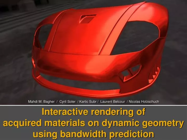
Mahdi M. Bagher / Cyril Soler / Kartic Subr / Laurent Belcour / Nicolas Holzschuch. Interactive rendering of acquired materials on dynamic geometry using bandwidth prediction. from Wikipedia. Illumination. BRDF. Shading.

E N D
Mahdi M. Bagher / Cyril Soler / Kartic Subr / Laurent Belcour / Nicolas Holzschuch Interactive rendering of acquired materials on dynamic geometryusing bandwidth prediction
fromWikipedia Illumination BRDF Shading • Direct reflection under distant illumination with no visibility and global illumination effects • Rendering an image is computationally expensive.
BRDF measurement Gantry [Matusik2002] Phong shading Measured “Color-Changing-Paint-3” Acquired Materials • Using measured materials • photo-realistic rendering • large memory footprint (33MB for a single isotropic BRDF) • Not suitable for real-time rendering
Monte Carlo approximation to the shading integral Importance sampling less noisy Data driven reflectance no analytical importance function pre-computed Importance samples Monte Carlo Sampling Monte Carlo sampling BRDF importance sampling
Dealing with two types of sampling Reconstruction sampling in image space to render an image Integration sampling in the space of incident directions to shade each individual pixel Illumination BRDF Cosine Sampling
Shading is slow… How to speed-up shading? The Problem
What difference various materials make in rendering an image? Case Study Measured reflectance data from [Matusik2002]
BRDF Lobe [BRDFLab] Diffuse Materials • Diffuse materials • shading varies slowly across the image (low frequencies) • many integration samples for each pixel (wide BRDF lobe) Measured Teflon [Matusik2002]
Measured color-Changing-Paint3 [Matusik2002] BRDF Lobe [BRDFLab] Specular Materials • Specular materials • shading varies quickly across the image (high frequencies) • few integration samples for each pixel (narrow BRDF lobe)
Rendering is slow… How to speed-up shading? Can we exploit the coherency between Reconstruction samples… Integration samples… …for adaptive sampling? How to measure the coherency between samples? The Problem
Study the frequencies in the image As a function of what happens to the light Traveling from the light source to the camera Intuition
Light when traveling is affected by Travel through free space Object’s curvature Reflectance BRDF Texture Occlusion The Traveling Light
How to speed-up shading? By sparse sampling the image How to combine the sparse samples? Multi-resolution rendering and bi-lateral up-sampling By adaptive sampling for integration Our Contribution
Adaptive Integration samples Sparse reconstruction samples Our Contribution (Illustrated) , ∝the local maximum variations in the image ∝ the average variance of the shading integrand Multi-resolution shading and bi-lateral up-sampling Final shaded image
Direct reflection under distant illumination No visibility and global illumination effects Allow dynamic editable geometry Screen-space rendering in the context of deferred-shading Any shading model is possible Save more if shading cost is higher e.g. measured materials BRDF importance sampling Normal Assumptions
Related work Our technique The goal Sparse sampling for reconstruction Adaptive sampling for integration Validation The rendering algorithm Results and comparisons Extension: MSAA Conclusion / Future work Roadmap
[Heidrich&Seidel1999] [Kautz2002] [Kautz&McCool1999] [Ramamoorthi2002] [Claustres2007] [Wang2009] [McCool2001] [Latta&Kolb2002] Related Work GPU Rendering of Complex Materials
[Nichols&Wyman2009] [Nichols&Wyman2010] [Nichols2010] [Segovia2006] [Shopf2009] [Soler2010] Related WorkMulti-Resolution Screen-Space Algorithms
[Loos2011] [Sun2007] [Sloan2002] [Liu2004] [Loos2012] [Ramamoorthi2009] Related WorkPre-Computed Transport
Related work Our technique The goal Sparse sampling for reconstruction Adaptive sampling for integration Validation The rendering algorithm Results and comparisons Extension: MSAA Conclusion / Future work Roadmap
Sparse sampling for reconstruction ∝ maximum local variations (local bandwidth) Adaptive sampling for integration ∝ variance of the shading integrand Multi-resolution rendering and bilateral up-sampling. a single coarse-to-fine rendering pass Goal
Related work Our technique The goal Sparse sampling for reconstruction Local light-field definition Spectral Operations 2D local bandwidth Image-space local bandwidth Adaptive sampling for integration Validation … Roadmap
4D local light-field illustrated in 2D Central ray Space Angle Local Light-Field
Related work Our technique The goal Sparse sampling for reconstruction Local light-field definition Spectral Operations 2D local bandwidth Image-space local bandwidth Adaptive sampling for integration Validation … Roadmap
Spectral Operations • Spectral operations [Durand et al. 2005] [Durand et al. 2005]
Related work Our technique The goal Sparse sampling for reconstruction Local light-field definition Spectral Operations 2D local bandwidth Image-space local bandwidth Adaptive sampling for integration Validation … Roadmap
2D Local Bandwidth maximum local variations about a light path both in angle and space. 2D local bandwidth spatial angular 2D Local Bandwidth
One-bounce 2D bandwidth propagation Transport (from light to reflector) Reflection (BRDF & Texture) Transport (from reflector to pixel) Matrix operators on 2D bandwidth where Transport to image plane Transport to the surface Bandwidth at pixel p Reflection operator Illumination bandwidth Scale Curvature Mirror BRDF and texture Curvature Scale Propagating Local Bandwidth
Illumination environment map Reflectance Acquired isotropic BRDFs Textures Input Signals Grace cathedral [Debevec2001] Gold-paint[ Matusik2003]
Illumination environment map Purely angular bandwidth Reflectance Acquired isotropic BRDFs Purely angular bandwidth Textures Purely spatial bandwidth Input Signals’ Bandwidth Grace cathedral [Debevec2001] Gold-paint[ Matusik2003]
Discrete Wavelet Transform to compute bandwidth environment map and reflectance (BRDF & Texture) Discrete Wavelet Transform instead of WFFT wavelets are well localized both in space and frequency. Computing Local Bandwidth Daubechies 4 tap wavelet FFT Space Frequency
Local Bandwidth Examples Grace cathedral [Debevec2001] Angular bandwidth Gold-paint[ Matusik2003] Angular bandwidth
Related work Our technique The goal Sparse sampling for reconstruction Local light-field definition Spectral Operations 2D local bandwidth Image-space local bandwidth Adaptive sampling for integration Validation … Roadmap
We combine bandwidth from various incident directions to get the final bandwidth at a given pixel. Taking a max is too conservative, we take the weighted average instead. Bandwidth at each pixel Bandwidth estimate based on max Bandwidth estimate Rendered image Image-Space Bandwidth
Related work Our technique The goal Sparse sampling for reconstruction Adaptive sampling for integration Validation The rendering algorithm Results and comparisons Extension: MSAA Conclusion / Future work Roadmap
# shading samples∝sum of bandwidths, weighted by the illumination times reflectance squared. The sum is a conservative approximation of the actual variance of the shading integrand. Angular bandwidth arriving at the surface Angular bandwidth of the reflectance Variance of the Shading Integrand
Related work Our technique The goal Sparse sampling for reconstruction Adaptive sampling for integration Validation The rendering algorithm Results and comparisons Extension: MSAA Conclusion / Future work Roadmap
Estimated bandwidth Measured variance Estimated variance Measured bandwidth (WFFT) Validation of the Bandwidth and Variance
Related work Our technique The goal Sparse sampling for reconstruction Adaptive sampling for integration Validation The rendering algorithm Results and comparisons Extension: MSAA Conclusion / Future work Roadmap
Step 1 Compute g-buffers Load Illumination and reflectance bandwidth Step 2 Estimate bandwidth and variance Step 3 Mip-map bandwidth and variance Step 4 Shade and up-sample The Algorithm
Related work Our technique The goal Sparse sampling for reconstruction Adaptive sampling for integration Validation The rendering algorithm Results and comparisons Extension: MSAA Conclusion / Future work Roadmap
Result (Final Image) 4x MSAA (1609 ms)
Fast bandwidth/variance estimation (8 ms) (ms) Timings (ms)
Computation time scales linearly with the total number of shading samples Timings
Comparison with Reference Similar quality (2639 ms) Our algorithm (1015 ms) Similar time (906 ms)